Macros provide you with a great mechanism to create and develop your ICM environment and adjust it to your own needs (see also How do I customize my ICM environment. ). Very often a repeated series of ICM commands is used for dealing with routine tasks. It is wise not to retype all these commands each time, but rather to combine them into a bunch for submission as a single command. Several examples follow.

alignTwoSequences : interface macro to the `Align function

 alignTwoSequences seq_1 seq_2 s_aliName ("NewAlignment") s_comp_matrix ("") s_alignmentAlgorithm ("ZEGA") r_GapOpen (2.4) r_GapExtension (0.15) i_maxPenalizedGap (99)

A macro to provide the interface to the Align( seq1 seq2 .. ) function and allows one to change global parameters influencing its behavior. Arguments:

two sequences
s_alignmentName
s_comp_matrix ("default"|"gonnet"|"blosum45"|"blosum50"|"blosum62"|"dna"|"hssp"|"ident")
s_alignmentAlgorithm ("ZEGA"|"H-align")
r_Gap_Open (2.4)
r_Gap_Extension (0.15)
i_maxPenalizedGap (99)

Example:

read sequence msf "azurins.msf"
alignTwoSequences Azur_Alcde Azur_Alcfa "ali2" "blosum45" "H-align" 2.6 0.1 99

calcArea : calculating solvent accessible surface area

 calcArea as_

calculates solvent accessible area of each selection in multiple objects and stores it in a table. If a molecule is specified in a multi-molecular object, the surface area of an isolated molecule is calculated and other molecules are ignored. The area is reported in square Angstroms and the probe radius is assumed to be waterRadius .

Output: the macro creates table AREA . The empty comment field is added for user's future use. If the table exists, new rows are appended. Example:

read pdb "1crn"
 read pdb "2crn"
 calcArea a_*.1  # calculate area around 1st molecule in each object:
 show AREA
 #>T AREA
 #>-Selection---Total_Area--Comment----
    a_1crn.1    2975.9      ""         
    a_2crn.1    4681.2      ""

See also:

show area surface as1 [ as2 ] [ waterRadius=.. ] : the main command used in this macro. This command gives larger flexibility since it allows definition of the second selection of the vicinity for the calculation.
surface area
waterRadius

calcBindingEnergy: estimates electrostatic, hydrophobic and entropic binding terms

 calcBindingEnergy ms_1 (a_1) ms_2 (a_2) s_terms ("el,sf,en")

evaluates energy of binding of two complexed molecules ms_1 and ms_2 s_terms for the given set of energy terms s_terms. This macro uses the boundary element algorithm to solve the Poisson equation. The parameters for this macro have been derived in the Schapira, M., Totrov, M., and Abagyan, R. (1999) paper.
Example:

read object s_icmhome+"complex" 
 cool a_ 
 calcBindingEnergy a_1  a_2  "el,sf,en"

calcDihedralAngle: calculate an angle between two planes in a molecule

 calcDihedralAngle as_plane1 as_plane2

calculates an angle between the two planes specified by two triplets of atoms, specified by the as_plane1 and as_plane2 selections
An example in which we measure an angle between planes of two histidines:

build string "ala his his"  # we use another macro here 
 display atom labels 
 calcDihedralAngle a_/2/cg,nd1,cd2 a_/3/cg,nd1,cd2 
 Angle=  131.432612  deg. (in ).

calcEnsembleAver: Boltzmann average the energies of the stack conformations

 calcEnsembleAver r_temperature (300.) s_parameter ("Value(v_/2/phi)")

a macro showing an example of how to calculate a Boltzmann-weighted average given a conformational stack of conformation representatives. The stack may be formed as a result of a Monte Carlo simulation or created manually. The s_parameter string contains any expression returning the parameter to be averaged (e.g. "Value(v_/2/phi)" or "Distance(a_/2/ca a_/4/ca)" ).
Example:

build string "ala his his" 
 set vrestraint a_/*  # impose rotamer probabilities 
 mncallsMC = 5000 
 montecarlo           # a stack is formed with energies 
 calcEnsembleAver 300. "Value(v_/2/phi)"

calcMaps: calculate five energy maps and write them to files

 calcMaps s_fileNameRoot ("rec") R_box r_gridSize (0.5)

calculates five energy grid maps for the current object with the grid size r_gridSize in the 3D box volume defined by the R_box . The maps are saved to files with names s_fileNameRoot_gc.map s_fileNameRoot_gh.map etc. and are deleted upon return from the macro. Be careful with selecting a box. You may focus the box on the area of interest (e.g. Box( a_/55,66 , 7.) ). To use the maps read them in, rename to m_gc m_gh, etc. and set terms "gc,gh,ge,gb,gs" . If you determined the box interactively you may just use the Box () function without arguments (it returns the parameters of the graphical box).
Example:

read object s_icmhome+"crn" 
 calcMaps "crn" Box( a_/15 4. ) 0.6 
 read map "crn_ge" 
 rename m_crn_ge m_ge  
 display m_ge {1 2 3 0 4 5 6} 
# the maps can be used in another session

Calculating the matrix of pairwise percent identities between sequences of from a multiple sequence alignment.

 calcPairSeqIdsFromAli ali l_original (yes)

calculates a pairwise sequence identities and returns them in two forms: as a table of pairs and as a matrix. Note:This macro is now obsolete and since the same result can be achieved with the Distance function. Example

read alignment "aln" name="aln"
 n=Nof(aln)
 mids = 100*(Matrix(n,n,1.) - Distance(aln ))  # the pairwise seq. identities
 t = Table( mids, Name(aln), Name(aln) )  # to convert the matrix into pairwise table
 t = Table( mids, index )  # a simpler version with i,j

Prerequisites, Input Arguments and Options

parameter	explanation
ali_	a multiple (or pairwise) sequence alignment
l_original	a parameter that determines if pairwise alignments are extracted from the multiple alignment as is ( `no` ), or pairs of sequences are realigned to avoid influences of other sequences ( `yes` ). We recomment to use the `yes` value.

Algorithm

each of the n&mult;(n-1)/2 , where
sequence identity is calculated as the number of identical columns in the alignment divided by

Output

variable name	explanation
`seq_ids` table	contains names of two sequences and sequence identity, `.seq1` `.seq2` , `.ident`
`seq_ids_mat` matrix	n x n matrix of pairwise identity values

Example

read alignment s_icmhome+"sh3.ali"
calcPairSeqIdsFromAli sh3 yes
show M_out
show T_out

See also:

alignment
Score ( ali2 identity )
Distance ( seq1 seq2 identity )

calcSeqSimilarity calculate sequence similarity according to an alignment

 calcSeqSimilarity aln s_refSeqName|i_refSeqPosInAli l_selection (no)

this macro returns a table, SeqSimilarity, with sequence identities with respect to the specified reference sequence ( s_refSeqName or i_refSeqPosInAli ). If a block of positions is selected (e.g. by selecting the binding site, or directly in the alignment editor), additional columns will show sequence similarity in the selected positions.

calcPepHelicity: calculate average helicity of a peptide from trajectory frames

 calcPepHelicity s_movieName r_temperature (300.)

a macro showing an example of how to calculate the helicity of a peptide structure given an ICM trajectory file of the conformations accepted during a Monte Carlo run. A simulation using montecarlo trajectory option is a prerequisite for this macro. A good script prototype can be found in the $ICMHOME/_folding file. The trajectory option saves each accepted conformation to a trajectory file. The secondary structure of all transient conformations is assigned with the assign sstructure command.
Example:

% _folding  # run the _folding script with the trajectory option. 
% icm 
 read object "mypep"  # the name of your peptide object 
 calcPepHelicity "mypep" 600.

calcProtUnfoldingEnergy: rough estimate of solvation energy change upon unfolding

 calcProtUnfoldingEnergy ms ( a_1 ) i_mncalls ( 100 )

calculates an octanol/water transfer solvation energy for the given # conformation as compared to an extended chain conformation.

calcRmsd: calculate three types of Rmsd between protein conformations

 calcRmsd rs_1 (a_1/*) rs_2 (a_1/*)

calculates Ca-atom, backbone-atom, and heavy-atom RMSD for two input residue selections. The main effort in this macro is to take the internal symmetry of amino-acid sidechains into account.
For example, two phenylalanines related by the 180 degrees rotation of the xi2 angle are identical, but will have a non-zero Rmsd(a_1./phe a_2./phe) because cd1 and ce1 of one selection lay on top of cd2 and ce2 atoms of the second selection, respectively. To calculate this Rmsd correctly, we need to find the rotation The following residues have internal symmetry (or pseudo-symmetry): leu,tyr,phe,asp,glu,arg,val.

calcSeqContent

 calcSeqContent S_sequenceNames

analyzes amino acid composition of the input sequence or sequences. Specify quoted sequence name, pattern (e.g. "*_HUMAN" ) or "*" for all sequences.
Example:

read sequence s_icmhome+"seqs" 
calcSeqContent "*"   # matches names of all sequences 
 .. 
 Statistics for 3 sequence(s): Azur_Alcde Azur_Alcfa Azur_Alcsp 
 AA   N   %   Expected  
 A   42 10.34   7.85 
 C    9  2.22   2.55 
 ... 
 
calcSeqContent "*de"  # sequences ending with 'de' 
 Statistics for 1 sequence(s): Azur_Alcde 
 Res  N   %   Expected  
 A   20 13.42   7.85 
 C    3  2.01   2.55 
 D    8  5.37   5.17 
 E    6  4.03   6.95

The columns are as follows:

One-letter amino-acid code
The total occurrence of the amino acid
Relative percentage occurrence in the given set of sequences
Expected mean occurrence of the amino acid in proteins

convertObject : creating a full atom model with types and charges from the source PDB file

 convertObject ms (a_) l_delete_water (yes) l_optimize_hydrogens (no) l_replace_the_original (no) l_display (no) l_optimize_his (yes) l_maskMissing (no) l_assignHeteroCharges (yes) s_options ("") auto

This macro converts a non-ICM object (e.g. PDB structure) into and ICM object and performs some additional refinements. Input: a selection of molecules (e.g. a_b,c ) and the following arguments:

l_delete_water (yes) : automatically deletes all waters
l_optimize_hydrogens ( no ) : performs global optimization of hydrogens for best hydrogen bonding network
l_replace_the_original ( no ) : keeps the same name as the original object and deletes it
l_display ( no ) : displays the converted object
l_optimize_his (--yes) : His protonations states will be tried, An and Gln flips will be tried and Cys in the the vicinity of Zn, Cu, Fe and Co to cym
l_maskMissing (no) : ICM will always add missing atoms for known residues. When l_maskMissing = yes these atoms will be masked off (hidden). They will be excluded from simulations, maps for docking etc.. This is for side-chains only it will not fill gaps in the backbone.
l_assignHeteroCharges (yes) : will set ligand charged state according to Molsoft's pKa model.

There are also some string options which can be added but must be space separated (e.g "water=tight tautomer amino_name_fix")

"tautomer" : optimize ligand tautomer. For each ligand (hetero a_H), different tautomeric forms are generated and their energies are evaluated using the "hb, vw, 14, el" terms in the context of other chains. The lowest-energy tautomer is then selected as the preferred form.
"amino_name_fix" : Automatically fix side chain and backbone atom names.
"water=tight" : ICM will keep waters making 3-4 hbonds.
"water=tight2.5" : ICM will delete loose waters making 0-1 hbonds with the receptor or ligand. This option will overwrite any l_delete_water setting. The classification of water molecules in ICM is determined by an empirical hydrogen-bonding potential score, where a higher score reflects a greater number of stable interactions. In this system, "tight" waters require a score above 5.0 (typically 3–4 bonds) and "intermediate" waters fall between 2.5 and 5.0, while "loose" waters score below 2.5—representing only 0–1 hydrogen bonds—and are generally removed to focus on structurally significant molecules.

For example if you are reading in a protein structure prepared in a different software and you do not need to add hydrogens and optimize or make any changes you can use:

 convertObject a_ no no no no no no no

or if you want to convert to an ICM object, and optimize hydrogens, His, Asn, Gln and add missing side-chain atoms and keep tight waters and optimize ligand tautomers you could use:

 convertObject a_ no yes no no yes no no "water=tight tautomer"

The procedure will do the following :

deletes water molecules (includes Deuteriorated water) if the 1st argument is yes
deletes the secondary alternative positions of atoms marked in the PDB (note that sometimes the alternatives are not marked and are deposited as concurrent independent molecules, e.g. two overlapping ligands in "1abe" )
it will built hydrogens based on residue library ( icm.res ) or valency/formal charge rules.
delete ambiguous covalent bonds with some metals according to the ICM and MMFF force field (e.g. around Fe ).
assign formal charge of -1 to atoms of MMFF type 4 and nitrogens next to Fe and deprotonate then accordingly
fix atoms of type 226 and MMFF type 15 around Zn (includes deprotonated Cysteines).
assign MMFF and ICM atom codes, and partial charges using the formal charges, MMFF types and bond charge increment scheme.
if heavy atoms that were missing in the PDB (due to the lack of density), they will be added according to the residue name and assigned zero occupancies.
in the converted object,
the following residues will be further optimized:
- His : three protonation states and two rotations will be tried and the residue will be renamed according to its subtype: hie (epsilon tautomer) or hip (+)
- Asn and Gln (a 180 deg. flip will be tried)
- Cys in the vicinity of Zn, Cu, Fe and Co to cym
if the 2nd argument is yes : (i) the atoms that were missing and/or atoms with occupancies ≤ 0.1 will be globally optimized to avoide clashes. (ii) the hydrogens will be systematically rotated for best energy
it also sets selftethers for the atoms with a non-ICM prototype. Later one can use term ts for restrained minimization.

Output:

the converted object. The original object is not changed unless the 3rd argument was yes .
the r_residualRmsd variable

Selection tags ( Select ( as tag ) returns the selection ) :

"built" -heavy atoms that were missing in a pdb (e.g. some lys and arg in 1qz5)
"shifted" -atoms that shift after conversion (e.g. silly lysines in 1qz5)

The macro returns r_residualRmsd value containing the Rmsd of the model atoms from the equivalent template atoms (the same value is returned by the convert command in r_out ). If this residual is greater than 0.5 , it usually means some problems with the conversion (e.g. unusual residues, missing parts, etc.).

This macro can be found in the __macro file or viewed using the edit command. It calls two other macros:

optimizeHisProAsnGlnCys (in _macro file )
optimizeH_zeroOcc (in _macro file )

Example:

read pdb "1abe"
  convertObject a_1,2 yes yes yes no
  show r_residualRmsd

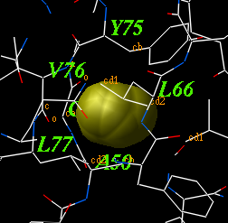
icmCavityFinder: analyze and display cavities

 icmCavityFinder as ( a_A ) r_minVolume ( 3. )

calculates and displays cavities in a molecular structure. These cavities are sorted by size, and displayed. To display the transparent outer shell edit the macro and activate this feature.
The r_minVolume parameters defines the volume of the smallest retained cavity. Increase it if you want only large cavities.
For each cavity this macro calculates volume V (in square Angstroms), area A and an effective radius R (compare it with the radius of a water molecule of 1.4A).

The icmCavityFinder macro uses two powerful features of ICM-shell:

a grob with analytical molecular surface ( a.k.a. skin ) of the selected atoms can be built using the make grob skin as_ as_ "g_skin" command.
this grob can be divided into the separate grobs with the outer shell and all the inner cavities with the split g_skin command.
icmCavityFinder also uses the Volume(g) and Area(g) functions to measure volume and area of the cavities, as well as the Sphere( g_ r_radius ) function to select atoms and residues around any grob.

Example:

read object s_icmhome+"1qoc" 
 delete a_w*  # remove water molecules 
 icmCavityFinder a_1 yes 4. 
   3  deleted 
  Info> finished surface search, n_of surface atoms = 744 
  Surface .................................................. 
  Info> finished basic surface element calculations 
  Info> Estimated vertex number = 335800, actual = 184896 
  Info> packing vertices... sorted... done! 
  Info> skin grob "" created (solid model: 32197 point 
  Info> 3 grobs   ...   created 
 Shell  1: V=11039.291805 A=4525.876702 
  Warning> Volume() may be improperly calculated: env 
 CAVITY 2: V=25.253718 A=44.282805 R~1.710848 -------------- 
 - Num  Res. Type ----{SS Molecule}-- Object - sf - sfRati 
    26  ile   Amino    I H  m            1qoc     0.0  0.00  
    53  leu   Amino    L E  m            1qoc     0.0  0.00  
    58  val   Amino    V _  m            1qoc     0.0  0.00  
    76  val   Amino    V E  m            1qoc     0.0  0.00  
    87  val   Amino    V E  m            1qoc     0.0  0.00  
    89  ile   Amino    I E  m            1qoc     0.0  0.00  
 ...

dsCellBox: displays crystallographic unit cell

 dsCellBox os (a_)

displays unit crystal cell box for the specified object os_ generated according to crystal symmetry parameters. This tiny macro extracts the cell from the object using the Cell function and makes a grob out of this array with the Grob function.

macro dsCellBox os_ (a_) 
  gCell = Grob ("cell" Cell(os_)) 
  display gCell magenta 
  keep gCell 
endmacro

findSymNeighbors: cell and crystallographic neighbors

 findSymNeighbors as ( as_graph ) r_radius (7.) l_append (no) i_extend_by (2) l_keepEntireChain (no) l_display (yes)

finds and builds symmetry related molecules around the input selection. The symmetry related atoms are generated according to the crystallographic symmetry group and cell dimensions.

Prerequisites and Arguments

a PDB entry or an icm-object that contains the information about the crystallographic unit cell and symmetry .
as_ ( default: as_graph ) : a source selection around which the symmetry neighbors are examined.
r_radius (7.) : the vicinity
l_append (no) : by default a separate object is created with all transformations. If yes the object with symmetry related atoms is added to the source object
i_extend_by (2) : if the next argument is no, the residue ranges that are within r_radius will be extended by the specified parameter and all the other (distant) residues will be deleted
l_keepEntireChain (no) : if this flag is yes the entire chain in which a proximal symmetry related atom is found will be kept, otherwise only the close residues (corrected by i_extend_by) will be kept
l_display (yes) : displaying the results.

The algorithm

The entire asymmetric unit is multiplied according to the Symgroup
then 26 additional cells (3*3*3-1=26) are generated around the current one.
the content is shifted to the 26 cells
the selection in the r_radius vicinity is make at the residue level and is extended by i_extend_by along the chain.
either entire molecule ( l_keepEntireChain is yes ) or the fragments are merged to the same object
the output variables are generated

The output

a single new object with the symmetry related neighbors (if l_append is no , otherwise it is appended to the existing object )
nSymNeighbors integer returns the number of symmetry related groups of atoms that were transformed
R_symTrans cancatenated transformation vector with 1+nSymNeighors sections of 12 elements (see transformation vector ). The first section is identity transformation.
S_neighborAtoms is a sarray with 1+nSymNeighbors residue selections in each transformation (skip the first one, the self selection)

Example:

read pdb "2ins"
findSymNeighbors a_1,2 5. no 2 no no  # a_2insSym. object with 14 fragments is created.
show nSymNeighbors, S_neighborAtoms
 7
 >S S_neighborAtoms
 a_2ins.1:2,5/*|a_2ins.c/^N21|a_2ins.d/^G8:^S9,^V12:^E13,^Y16,^G20:^K29
 a_2ins.5/*|a_2ins.b/^S9:^H10|a_2ins.c/^L13|a_2ins.d/^V2:^Q4,^L6,^A14,^Y16:^E21
 a_2ins.b/^K29
 a_2ins.5/*|a_2ins.b/^H10
 a_2ins.c/^G1,^E4|a_2ins.d/^P28:^A30
 a_2ins.b/^R22
 a_2ins.c/^A8:^V10|a_2ins.d/^N3,^H5
 a_2ins.c/^G1,^N18:^Y19,^N21|a_2ins.d/^F25,^K29:^A30

dsChem : chemical style display

 dsChem as (a_)

3D display of the input atom selection in chemical style and on white background.
If you want to 'flatten' the molecule you can perform a procedure from the following example:

build string "trp"      # you need an ICM object  
 tzMethod = "z_only" # tether to the z-plane 
 set tether a_       # each atom is tethered to z=0  
 minimize "tz"       # keep the cov. geometry

dsCustom: extended display and property-coloring

 dsCustom as (a_) s_dsMode ("wire") s_colorBy ("atom") l_color_only (no)

Displays the specified representation ( "wire", "cpk", "ball", "stick", "xstick", "surface", "ribbon" ) of a molecular selection and colors the selection according to the following series of features:

atom type ( s_coloringType="atom" ),
residue type ("residue"),
unique molecules ("molecule"),
secondary structure type ("sstructure"),
N-to-C-terminal chain course (NtoC""),
B-factors ("bfactor"),
electric charges ("charge"),
solvent accessibility ("accessibility"),
residue polarity ("polarity"),
residue hydrophobicity ("hydrophobicity")

dsPropertySkin: display molecular surfaces colored by properties essential for binding

 dsPropertySkin as_sel (a_) l_wire (yes) l_biggestBlobOnly (no)

displays essential properties of molecular surfaces which are essential for binding small ligands, peptides or other proteins.
The first argument is a selection of atoms involved in the surface calculation. The second argument allows you to display the surface as:

skin ( l_wire=no ), or
wire ( l_wire=yes )
l_biggestBlobOnly: splitting and keeping the biggest blob only

The color code:

white - neutral surface
green - hydrophobic surface
red - hydrogen bonding acceptor potential
blue - hydrogen bonding donor potential

Example shown:

read pdb "1a9e" 
 delete a_w* 
 convert    # convert to ICM for map calculations 
   # select receptor atoms 9. away from the peptide with Sphere 
 cool a_    # display ribbon 
 dsPropertySkin Sphere( a_3 a_1 9. ) yes no
   # adjust clipping planes for better effect 
 write image png

Interactive surface display under GUI The same can be performed interactively on ICM objects with the popup-menu:

display your ICM object
switch selection level to residue (R)
select region with selection box or lasso
click on the right mouse button over one of the selected residues
selected Display and then Property Skin
it creates grob g_recSkin which can then be undisplayed and further manipulated

calcEnergyStrain: analyzing energy strain in proteins

 calcEnergyStrain rs ( a_/A ) l_colorByEnergy (yes) r_max (7.)

calculates relative energy of each residue for residue selection rs_ ; and colors the selected residues by strain ( if logical l_colorByEnergy is "yes" ). The r_max argument determines the range represented by the color gradient (i.e. residues strained beyond 7. will still be shown in red).
This macro uses statistics obtained in the Maiorov, Abagyan, 1998 paper.
Example:

read object s_icmhome + "crn" # an ICM object 
 calcEnergyStrain a_/A yes 7.
 show ENERGY_STRAIN

Calculate normalized 'area under curve' for the hit enrichment histogram vs rank or square root of hit rank

 calcRoc R_scores L_01labels r_score_error (0.) l_linear_auc (no) l_keep_table (no) l_showresults (yes)

compute the normalized measure of the recognition strength of the provided score ( R_scores ) given a matching array of zero and one labels for 'noise' and 'signal' respectively. Lower scores are considered better (comes from energy), invert the sign of the scores otherwise. Example: scores { 2.1 4. 3. 44.} and labels {1 0 0 0} correspond to a perfect recognition since 2.1 is the lowest score.

The normalized measure returns the value of 100. for any perfect separation of signal from noise and values close to zero for a random subset of noise. The normalized measure is based on the area under curve in the following axis: the number of signal records in the top N scores versus the record rank (or the square root of it). The rank is defined as the order in a sorted array. The normalized measure is the following:

AUC..normalized = 100*( AUC - AUC_random )/(AUC_perfect / AUC_random )

Input

a real array of N Scores R_scores
an integer array of N zero or one labels
an error of the score values
a flag to to calculate the linear version of AUC (the square root is the recommended default, however)
a flag to keep the resulting table
a flag to print the NSA values (otherwise

Algorithm

a table of N scores and N labels is built
the table is sorted by scores
a histogram of percentage of signal rows in M best scores is plotted
the X-axis of the histogram is transformed as follows: X = Sqrt(100.*M/N) (or X = 100.*M/N for the linear version)
an area under the resulting curve AUC is calculated and divided by the size of the X axis. The resulting number is between 0. and 100.
the random and the perfect AUC values are calculated
the normalized value is calculated as: AUC..normalized = 100*( AUC - AUC_random )/(AUC_perfect / AUC_random ) .
if the r_score_error parameter is greater than zero, the scores are modified with the random Gaussian noise and the nosauc values are computed every time. Rms and mean are calculated and stored in the header of the tabauc table.

OutputIf the l_keep_table flag is set to no, the four values are returned as R_out[1:4].

R_out[1] returns the NSA value
R_out[2] returns the mean NSA value after the score values have been modified with Gaussian noise 35 times
R_out[3] returns the standard error of the NSA value after introducing the Gaussian noise.
R_out[4] returns the Normalized Median Rank (the median rank from 1 to 100) of the positives.

Otherwise a table called tabauc is created.

tabauc table that can be used to plot the enrichment (if l_keep_table is defined as yes ). It contains arrays: A (labels), S (score) , R (the last randomized score), X (the relative Sqrt(rank) or rank), and N (the cumulative enrichment). Plot N vs X for a AUC plot.
tabauc.nosauc ( a real value ≤ 100. ) : normalized area under curve in normalized %hits vs sqrt( %rank ) axes. Values around zero or negative are indicative of no recognition. The perfect recognition corresponds to a value of 100.
nosauc_ave (real) : if r_score_error is not zero, it gives an average nosauc upon many Gaussian randomizations of the scores
nosauc_rms (real) : if r_score_error is not zero, it gives an rmsd of nosauc upon many Gaussian randomizations of the scores
nmr (real) : returns the Normalized [0. to 100.] Median Rank of the positives. E.g. if there are 5 binders and 1000 nonbinders, it will return the rank of the 3rd positive (3 is the median in a set of 5), normalized to a value from 0. to 100.
type (string) : contains "linear" or "sqrt"

Example:

N=1000; n=100
calc_nosauc Random(0.,1.,n,"gauss")//Random(3.,1.,N-n,"gauss") Iarray(n,1)//Iarray(N-n) 0.2 yes no
show R_out
show tabauc.nosauc, tabauc.nmr
# select columns X and N and plot the enrichment curve.
# play with the parameters

chemSuper3D

 chemSuper3D os_in os_template l_optimize (no) l_display (no) l_all (no) auto

performs a sequential flexible superposition of multiple molecules in the os_in selection on a single rigid template os_template . For static superposition, use superimpose chemical .

Prerequisites and Input

several objects with chemical hetatm molecules
os_in : contains one molecule per object

Parameters and options

l_all - option of the find molecule sstructure command. By default l_all = no only one largest match is used.
l_optimize - currently inactive
l_display - displays the result

Output

Flexible molecules superimposed on the template.

See also:

superimpose ( superimpose chemical for rigid superposition)
find molecule sstructure (find the maximal common substructure )

icmPmfProfile

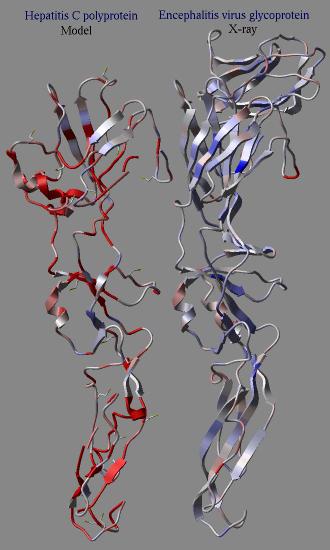
 icmPmfProfile os ( a_ ) l_accessibilityCorrection (yes) l_display ( no )

calculates a statistical energy of mean-force for each residue of a provided object. This energy is calculated with the "mf" parameters defined in the icm.pmf file. The residue energies are then normalized to the expected mean and standard deviation of the same residue in real high resolution structures. The mean energy value can be calculated as a function of its solvent accessibility if l_accessibilityCorrection is set to yes.
The calculated table contains residue energies and accessibilities. These values can be used to color residues of the molecule according to those values. In an example shown here we build a model (using the build model command of HCV protein on the basis of another viral coat protein. Then the profile was calculated for the model and the original structure. The calculation clearly shows the problematic regions of the model (the red parts) while the source structure looks quite reasonable.

dsPrositePdb

 dsPrositePdb ms (a_*) r_prositeScoreThreshold (0.7) l_reDisplay (no) l_dsResLabels (yes)

Finds all PROSITE pattern-related fragments in the current object and displays/colors the found fragments and residue labels.

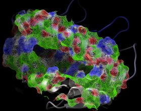
dsRebel: surface electrostatic potential

 dsRebel as (a_*) l_assignSimpleCharges ( no ) l_display (no)

generates the skin representation of the molecular surface colored according to the electrostatic potential calculated by the REBEL method (hydrogen atoms are ignored). The coloring is controlled by the maxColorPotential and TOOLS.rebelPatchSize parameter. This macro uses a simplified charge scheme and uses only the heavy atoms for the calculations for the sake of speed.

See also:

color grob potential [heavy]
rebel
maxColorPotential
Electrostatic troubleshooting section in rebel

dsSeqPdbOutput : visualize the sequence similarity search results

 dsSeqPdbOutput s_projName ("brku") l_resort (no)

Goes through a list of PDB hits resulting in find database command and displays alignment(s) of the input sequence(s) with the found PDB structures and SWISSPROT annotations.

dsSkinLabel

 dsSkinLabel rs (a_/*) s_color ("magenta")

For all residues specified by the input residue selector, rs_, displays residue labels shifted toward the user to make the labels visible when skin representation is used.

dsPocket and dsPocketRec

 dsPocket ms_ligand (a_H [1]) s_GrobName ("") l_overwrite (yes) l_ds_xstick_hb_labels (no)

 dsPocketRec ms_ligand (a_H [1]) ms_receptor (a_!H ) r_margin (6.5) s_GrobName ("") l_overwrite (yes) l_ds_xstick_hb_labels (no)

display the receptor pocket around the selected ligand ms_ligand. Only the largest contiguous pocket surrounding the ligand is retained for clarity. Macro also colors the molecular surface by hydrogen bonding potential and hydrophobicity if receptor is as ICM object. Best used with the ligand shown in cpk, if the ligand is small.

The first macro ( dsPocket ) is trying to guess what the selecting of atoms for the binding pocket is. Then it calls dsPocketRec The second macro ( dsPocketRec ) has identical arguments plus explicit receptor selection.

The dsPocket guess about the receptor:This is the order of guesses about the selection of the binding pocket molecules:

The macro first tries to see if there is a "receptor" of the ICM type specified by the interactive 3D editor ( the Ligand tab of the GUI tools)
Then it tries to get all molecules from the same object as the ligand selection except the ligand and water molecules
if step 2 fails, it tries to find the first ICM object among those displayed that is within a 7A vicinity of the ligand

Prerequisites and arugments of the dsPocketRec macro

a ligand (can be a selection in an object) and selecting of molecules interacting with the ligand. Both ligand and binding pocket can belong to an ICM or non-ICM (raw PDB) objects.
r_margin : the cutoff distance from the ligand atoms for the pocket calculation
s_GrobName : the preferred name for the pocket grob object.
l_overwrite logical will overwrite the previous pocket grob with this name if yes .
l_ds_xstick_hb_labels logical will display the contact residues in xstick, hydrogen bonds and residue labels

The procedure

the analytical molecular surface ( aka skin ) is computed as a grob object consisting of triangles.
the surface is split into contingous grobs and only the largest one is retained.
coloring: if the "receptor" object is of the non-ICM (PDB or Model) type it will get a uniform lightcyan color.
coloring for the pockets from ICM objects: the grob is initially colored white. Then some hydrophobic areas are colored green, the hydrogen bond acceptor surfaces as red and the hydrogen bond donors as blue .
coloring the movable binding pocket side chains. The carbons of movable side chains in the 4A vicinity of the ligand are colored pink .
the residues in the pocket are labeled.

Output

the grob (mesh) object with specified name colored by pharmacophoric properties if the selection of binding molecules belonged to an ICM object
the grob will be displayed as a transparent smooth object. You can change the type of display by right clicking on the display icon in the GUI WorkSpace.

These macros can also be used to show protein-protein interface.
Example:

read object s_icmhome+"complex" 
 cool a_ 
 dsPocket a_1 "" yes  # shows the surface of a_1

This macro replaces dsSkinPocket and dsSkinPocketIcm macros.

dsStackConf

 dsStackConf as (a_//n,ca,c) i_from (1) i_to (Nof(conf)) s_superimpRes ("*")

displays superimposed set of conformations from a conformational stack for given selection as_.

dsVarLabels

 dsVarLabels

displays color labels for different types of torsion variables.

ds3D

`ds3D auto M_dist S_names ({""}) S_comments ({""})` display 3D coordinates corresponding to an input square distance data matrix. Relative errors (in percent) of embedding to 3D space are in R_out: first entry is for the total error, next three are for X, Y and Z coordinates.
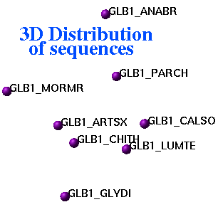
	Representation of inter-sequence evolutionary distances in three-dimensional space

dsXyz : display

 dsXyz M_3coor

displays points from the N_atoms x 3 matrix of M_3coorin 3D space as blue balls. The origin of the Nx3 matrix is not important. The macro creates an object called a_dots. In this object each dot is a one-atom residue called 'dot'. The atom type is arbitrarily assigned to oxygen, and the atom names are 'o'.
One can further manipulate this object, e.g. color a_/12:15/o green .
An example in which we generate sparse surface points at vwExpand distance around a molecule and display them.

build string "ala his trp" 
 mxyz = Xyz( a_ 5. surface ) 
 display skin white 
 dsXyz mxyz   
 color a_dots. red

find_related_sequences macro: identify similar and superposable chains in multiple objects

 find_related_sequences auto ms (a_*.A)

identifies pairs of molecules (chains) with similar sequences in the input selection. (see also Select( seq .. ) ) Input and arguments

one or several objects with two or more amino-acid chains (molecules)
a selection of more than one molecules with more than five amino-acids

The procedure

* for each pair of amino-acid chains in all objects the following:

extract sequences and align them using alignMethod ="ZEGA", record sequence identity ( seqid )
superimpose them by using this alignment and calculated heavy atom ( rmsd )
record all pairs with the alignment probability value less than 0.0001 or alignment sequence identity > 90%
add a pair to the related_sequences table

Output

related_sequences table with the following columns: name1 name2 len1 len2 seqid rmsd consensus
the table is active: if you double click on a pair two related chains will be selected

Example:

read pdb "1arb"
read pdb "1arc"
find_related_sequences a_*.*
show related_sequences

findFuncMin

 findFuncMin s_Function_of_x ("Sin(x)x-1.") r_xMin (-1.) r_xMax (2.) r_eps (0.00001)

minimizes one-dimensional functions provided as a string with the function expression. The macro uses successive subdivision method, and assumes that the function derivative is smooth and has only one solution in the interval
Example:

findFuncMin "Sin(x)*x-1." , -1. 2. 0.00001 
 -1.000000 < x < 0.500000 
 -0.250000 < x < 0.500000 
 -0.062500 < x < 0.125000 
 .... 
 -0.000004 < x < 0.000008 
 -0.000004 < x < 0.000002

findFuncZero

 findFuncZero s_Function_of_x ("Exp(-Exp(-x))-0.5")  r_xMin (0.) r_xMax (1.) r_eps (0.00001)

finds a root of the provided function of one variable with specified brackets with iterations. E.g.

findFuncZero "x*x*x-3.*x*x" 1. 33. 0.00001 
 -> x=17.000000  F=4046.000000 
 -> x=9.000000  F=486.000000 
 -> x=5.000000  F=50.000000 
 -> x=3.000000  F=0.000000

Determining selection axis and making an arrow.

 makeAxisArrow rs ( a_/10:18 ) i_length (10) r_radius ( 0.12 ) r_head_width_ratio ( 2. )

this macro determines the direction make an arrow with specified parameters. Input and arguments:

rs_ a contiguous residue selection (usually a strand or a helix, but it will work anyway).
i_length (10) : if 0 is specified the length will be determined from the selection
r_radius ( 0.12 ): arrow radius in Angstroms (see GROB.arrowRadius )
r_head_width_ratio ( 2. ) : relative expansion of the arrow radius for the arrow head (see GROB.relArrowHead )

Output

an average helical angle is reported
a grob with name starting from "axis_" and molecule name , e.g. axis_m

Example:

read pdb "1crn"
display ribbon
makeAxisArrow a_/23:30 10 0.2 2.1
color axis_m blue

modifyGroupSmiles

 modifyGroupSmiles as_group s_Group l_reset_MMFF_types (yes) l_reassign_MMFF_charges (yes) l_optimize_geometry (no) auto

attaches a chemical group to the specified anchor atom. Input and Arguments

an ICM object of a chemical
as_anchor : an atom to be modified, frequently a hydrogen. If a heavy atom is specified instead of a specific hydrogen, the first hydrogen will be used to determine the growth direction.
s_Group : the attachment point can specified as [atomName*] or just as *. The first atom is assumed to be the attachment point if the attachment is not explicitly specified. Example smiles: "C[C*](C=O)O" (the second atom is the attachment point), "C(C=O)O" the first carbon is taken.
l_reset_MMFF_types (yes) : flag to rest the types for all atoms in the molecule
l_reassign_MMFF_charges (yes) : reassign the chages
l_optimize_geometry (no) : uses MMFF minimization to improve geometry

Output

Modified molecule

morph2tz : generating sterically plausible intermediate conformation for conformational morphing

 morph2tz rs_loop ( a_/ ) i_nIter l_store_in_object (no) l_play_morph (yes)

this macro generates a stack of intermediate conformations for an fragment in an object. This intermediate conformations are obtained by a restrained minimization using the source and target structures, as well as the steric restrains.

Prerequisites and arguments

an ICM object in which a subset of atoms (including a special case of all atoms) is tethered to atoms in a different destination object. For example a DFG-in loop in a kinase tethered to a DFG-out conformation in another object. This set up can be prepared with the "modeler's view" GUI tool.
the rs_loop fragment of an ICM object (e.g. a_a/394:406 )
i_nIter is the number of intermediate conformations requested to be generated. Since the resulting stack of conformers can further be interpolated using the l_play_morph option ( and after the macro with the display stack command), this number does not need to be very big, say 10 to 50.
l_store_in_object (no) : this flag determines if the stack at the end is also stored inside the object. The default action is to generate a common stack .
l_play_morph (yes) : if yes the generated stack will be played in an interpolated fashion using the display stack command.

The algorithm

the key point is to have the destination coordinates compatible with the coordinates of the regions flanking the selection
the coordinates before and after the selected fragment are kept as is.
each intermediate conformation is generated by minimizing the van der Waals and torsion energy and differently weighted restrains to the source and destination coordinates. The energy terms used are the following "vw,14,to,ts,tz,rs" . Feel free to modify this command it you can tolerate a longer calculation and care about the quality of the intermediate conformations.
the generated minimized conformers are stored in the conformational stack
further interpolation between them can be done with the display stack command.

The output

The default output is a stack of conformations with i_nIter minimized intermediate conformations between the start and the finish.
If l_store_in_object flag was yes , the stack is also compressed and copied to the object

nice

 nice auto s_PdbSelection ("1crn") l_invert (no) l_wormStyle (no) l_append (no) l_nodisplay (no)

reads and displays a PDB structure in ribbon representation; colors each molecule of the structure by colors smoothly changing from blue (at N-terminus) to red (at C-terminus). The auto keyword allows one to skip N last arguments.
Example:

nice "365d"  # new DNA drug prototype 
 nice "334d"  # lexitropsin, derivative of netropsin

cool

 cool auto rs (a_) l_static (no)

similar to the macro nice above, but refers to a residue selection.

homodel

 homodel ali l_quick (yes)

homology modeling macro. The first sequence in the input alignment should contain the sequence of a PDB template to which the modeling will be performed. If flag l_quick is on, only an approximate geometrical model building is performed. You can also use the build model command directly.

loadEDS

 loadEDS s_pdb ("1mui") r_sigma (0.)

read the 2fo-fc map file with crystallographic electron density from one of three sources. (for fo-fc map use loadEDSweb ) The map named m_s_pdb (e.g. m_1crn ) is loaded from the Uppsala server or a local directory. If the macro ends up loading it from the web, it writes the map a local repository as s_pdb.map file for fast future access. To read the map file three locations are checked in the following order:

s_userDir + "/data/eds/" directory.
TOOLS.edsDir directory. This directory can be shared and have read permissions only.
the Uppsala EDS server. This is performed with the loadEDSweb macro.

The arguments

s_pdb ("1mui") : 4 letter pdb code. The resulting map will be 1mui.map for that code.
r_sigma (0.) : if not zero, a grob with the electron density contour is created.

The procedure

the 2Fc-Fo map for the entire crystallographic cell is uncompressed and loaded from a local directory or the server.
the map is contoured at the specified sigma level if sigma is non-zero. Keep it at zero for speed, unless you need the contours.
if a pdb object with the same name is present in the directory, ICM will contour only around the atoms of the object instead of creating the grob for the entire crystallographic cell.

The output

New files, if the map was downloaded from the web.

compressed s_pdb.map file in TOOLS.edsDir directory if it is write accessible
alternatively, compressed s_pdb.map file in s_userDir + "/data/eds/" directory

The following ICM shell objects:

map m_s_pdb
grob g_s_pdb
if matching pdb object is found (and it has some atoms selected), an extra smaller map is created around the selection for interactive sigma-level change.

loadEDSweb

 loadEDSweb auto s_pdbcode ("1mui") [ s_maptype ("2fofc") ]

downloads 2fofc (or other s_maptype) map from the Uppsala electron density server "http://eds.bmc.uu.se/"Creates a map object m_s_pdbcode . This macro can be used to load Fo-Fc maps ( s_maptype "fofc" ) This macro is used by the loadEDS macro.

Example:

loadEDSweb "1mui" "2fofc"
display m_1mui
# or 
loadEDSweb "1mui" "fofc"

makeIndexChemDb

 makeIndexChemDb s_dbFile ("/data/acd/acd.mol") s_dbIndex ("/inx/ACD") s_dbType ("mol2") S_dbFields ({"ID"})

Creates and saves an index to a small compound database existing in standard "mol" or "mol2" formats (specified by the s_dbType parameter). s_dbIndex defines full-path root name of several index-related files. String array S_dbFields specifies fields of the input database which are indexed by the macro.
An example in which we index the cdi.sdf file and generate the cdi.inx file in a different directory:

% icm 
makeIndexChemDb "/data/chem/chemdiv/cdi.sdf" "/data/icm/inx/cdi" "mol" {"ID"}

makeIndexSwiss

 makeIndexSwiss s_swiss (s_swissprotDat) s_indexName (s_inxDir+"SWISS.inx")

Creates and saves an index to the SWISSPROT sequence database (datafile s_swiss). s_indexName defines the root name of several index-related files with respect to ICM user directory, s_userDir.

makePdbFromStereo: restore 3D coordinates from a stereo picture

 makePdbFromStereo R_xl R_xr R_yl R_yr r_stereoAngle ( 6. )

transforms two stereo sets of two-dimensional coordinates in arbitrary scale into 3D coordinates. See also: How to reconstruct a structure from a published stereo picture .

makeSimpleDockObj

 makeSimpleDockObj os s_newObjectName

This macro builds an ICM object from simplified residues described in the residue library. The goal is to convert an all-atom molecular object into an object in simplified representation for fast docking calculations.

makeSimpleModel

 makeSimpleModel seq ali os

This macro rapidly builds a model by homology using simplified residues described in the residue library. Input data are the sequence of the model, seq_ and alignment ali_ of the model's sequence with the template object os_ .

mkUniqPdbSequences

 mkUniqPdbSequences auto i_identPercent ( 1 )

Creates a collection of PDB sequences with specified degree of mutual dissimilarity, i_dentPercent.

placeLigand: flexible superposition of a ligand to atom selection

 placeLigand ms_movable_ligand_ICM as_static_target_ICM r_effort (1.) l_display l_debug

placeLigand docks a ligand molecule in a single ICM object to the specified atom selection in ICM-converted objects. Selections of groups/ligand in multiple ICM Objects is allowed as a destination. If additional restraints/tethers are needed, use distance tool to define them. Tethers that are set directly via 'set tether' will be respected too. The macro saves a stack of preferred superposisions. No additiona entities/objects/maps are created. Parameters:

ms_movable : flexible (ICM) molecule to be moved to the destination selection
as_satic : atoms in one or multiple molecules in ICM-converted objects for superposition
r_effort : (default 1.) defines how rigorous/long the search is
l_display : display placement

Example:

read object s_icmhome + "biotin.ob" 
build smiles "CCCC(=O)[O-]" name="lig"
display xstick a_biotin,lig.
pause 
placeLigand a_lig. a_1.1 3.

plot2DSeq

 plot2DSeq ali_

generates a 2D representation of "distances" between each pair of sequences from the input alignment.

plotSeqDotMatrix

 plotSeqDotMatrix seq_1 seq_2 s_seqName1 ("Sequence1") s_seqName2 ("Sequence2") i_mi (5) i_mx (20)

generates an EPS file in which local sequence similarities between two sequences are shown in the form of a two-dimensional dot-matrix plot. Significance of local sequence similarities is shown by logarithm of the probability values and is calculated in multiple windows from i_mi to i_mx. The log-probability values are color-coded as follows: light blue: 0.7, red 1.0.

plotSeqDotMatrix2

 plotSeqDotMatrix2 seq_1 seq_2 s_seqName1 ("Sequence1") s_seqName2 ("Sequence2") i_mi (5) i_mx (20)

generates an EPS file in which local sequence similarities between two sequences are shown in the form of a two-dimensional dot-matrix plot. Significance of local sequence similarities is shown by ( 1. - Probability(..) ) values and is calculated in multiple windows from i_mi to i_mx. The ( 1 - P ) values are color-coded as follows: light blue: 0.7, red 0.99.

plotBestEnergies

 plotBestEnergies s_McOutputFile ("f1,f2") r_energyWindow (50.) s_extraPlotArgs ("display")

plots profile of energy improvement during an ICM Monte Carlo simulation. Data are taken from the MC output log file or files, s_McOutputFile. You can specify a single output file (e.g. "f1.results"), or several files, e.g. "f1.ou,f2.ou", or drop the default ".ou" extension, e.g. "f1,f2,f2".
This macro gives you an idea about the convergence between several runs.

plotFlexibility

 plotFlexibility seq i_windowSize (7)

calculates and plots flexibility profile for input sequence seq_ and smooths the profile with i_windowSize residue window.

plotCluster

 plotCluster M_distances S_names ({""}) s_plotArgs ("CIRCLE display {\"Title\" \"X\" \"Y\"}")

plot distribution of clusters. Arguments:

a square matrix of distances between n objects. For arrays it may be calculated with the Distance ( ) function (e.g. Distance(Xyz(a_//ca))). For angular RMSD the distance can be calculated from a matrix v of values of torsion angles for many conformations:

for i=1,n-1 
   di[i,i]=0. 
   for j=i+1,n 
            # takes care of -179 and 181, base 360 is the default 
      dif=Remainder(v[i]-v[j])    
            # angular RMSD 
      di[i,j]=Sqrt(Mean(dif*dif))   
      di[j,i]=di[i,j] 
   endfor 
 endfor 
 di[n,n]=0.

sarray of names for each of n points . Possibilities:
- the empty sarray: {""}. No name tags will be attached to each point
- Sarray(Count(n)) generates names like this: {"1" "2" "3" ... }
- user-defined: e.g. Name(a_*.) if each point correspond to an object
- manual: e.g. {"A" "compound X" "c"}
See also: arguments for the plot command.

plotMatrix

 plotMatrix M_data s_longXstring S_titles ({"Title","X","Y"}) s_fileName ("tm.eps") i_numPerLine (10) i_orientation (1)

generates combined X-Y plot of several Ys (2nd, 3rd , etc. rows of the input matrix M_data) versus the one X-coordinate, assumed to be the first row of the matrix. i_numberPerLine parameter defines the size of the plotted block size if the number of data points is greater then i_numberPerLine. i_orientation equal to 1 defines portrait orientation of the output plot, landscape otherwise.

plotRama and plotRamaEps

 plotRama rs

generates a residue table and three interactive plots for non-glycines, glycines and omega angles (see Tools/Analysis menu)

 plotRamaEps rs l_show_residue_label (no) l_shaded_boundaries (yes)

generates a phi-psi Ramachandran plot of an rs_ residue selection. If logical l_show_residue_label is on, the macro marks the residue labels. If l_shaded_boundaries is on, the allowed (more exactly, core) regions are shown as shaded areas; otherwise the contours of the core regions are drawn.

plotRose

 plotRose i_prime (13) r_radius (1.)

just a nice example of a simple macro generating "rose" plot.

plotSeqProperty

 plotSeqProperty R_property s_seqString S_3titles {"Y property","Position","Y"} s_fileName ("tm.eps") i_numPerLine (30) s_orientation ("portrait")

a generic macro to plot local sequence properties. Modify it for your convenience. Here is an example in which we plot residue b-factors along with the crambin sequence. s_seqString could be the sequence (e.g. String(1crn_m) ) or secondary structure, (e.g. Sstructure(1crn_m) ) or any other string of the same length as the sequence.

read pdb "1crn" 
 make sequence  
 b = Bfactor( a_/* ) 
 plotSeqProperty b String(1crn_m ) {"" "" ""} "tm.eps" 20 "portrait"

predictSeq

 predictSeq s_seq ("1crn_m") s_fileName ("plot") l_predictSstr (no) i_numPerLine (100)

prepSwiss

 prepSwiss s_IDpattern ("VPR_*") l_exclude (yes) s_file ("tm")

extracts all sequences from the SWISSPROT database which exclude ( l_exclude= yes ) or include ( l_exclude= no) the specified sequence pattern, s_IDpattern and creates a set of database files with the rootname s_file intended to use in the command find database.

printMatrix

 printMatrix s_format (" %4.1f") M_matrix (def)

prints matrix M_matrix according to the input format s_format.

printPostScript

 printPostScript s_ofPrinterName ("grants")

converts the current content of the graphics window to a PostScript file and directs it to the s_ofPrinterName printer.

printTorsions

 printTorsions rs (a_/A)

outputs all torsion angles of the input residue selection.

refineModel: globally optimize side-chains and anneal the backbone

 refineModel i_nRegIter (5) l_sideChainRefinement (no)

This macro can be used to improve any ICM model. The model can come from the build model command or the convert command or regul macro, etc. It performs

side-chain sampling using montecarlo fast
interactive annealing with tethers you have provided
second side-chain sampling to resolve the new problems resulting from the second step

To perform only the side-chain refinement, set the i_nRegIter argument to 0 .

regul

 regul rs (a_!W) s_ngroup ("nh3+") s_cgroup ("coo-") l_delete_water (yes) l_shortOutput (yes)

creates a regularized ICM-model of an input residue selection ( rs_ ) modified by the N- and C-terminal groups ( s_ngroup and s_cgroup, empty "" strings are allowed);

rdBlastOutput

 rdBlastOutput S_giArray

reads a set of sequences defined in a BLAST's output file, S_giArray from the NCBI database.

rdSeqTab

 rdSeqTab s_dbase ("NCBI")

reads a set of sequences listed in the ICM-table SR, an output of find database command, from the database defined by s_dbase.

remarkObj

 remarkObj

allows editing an annotation (comment) of the current object. Existing comment (if any) is read in an editor and after modification assigned to the object.

searchPatternDb

 searchPatternDb s_pattern ("?CCC?") s_dbase ("SWISS")

searches for the pattern in the sequences of the specified indexed database s_dbase.

searchPatternPdb

 searchPatternPdb s_pattern

searches for the specified pattern in pdb sequences taken from the foldbank.db file.
Example (first hydrophobic residue, then from 115 to 128 of any residues, non-proline and alanine at the C-terminus):

searchPatternPdb "^[LIVAFM]?\{115,128\}[!P]A$"

searchObjSegment

 searchObjSegment ms i_MinNofMatchingResidues (20) r_RMSD (5.)

for given molecule ms_ finds all examples of similar 3D motifs not shorter than i_MinNofMatchingResidues residues with the accuracy r_RMSD A in the ICM protein fold database.

searchSeqDb

 searchSeqDb s_projName ("sw1") S_seqNames ({""}) r_probability (0.00001) l_appendProj (no) s_dbase ("SWISS")

search the database s_dbase using query sequence(s) specified in S_seqNames. Found hits and their specs are collected in the output table file s_projName.tab. If logical flag l_appendProj is on data will be appended to the existing table. Similarity of hits to the query sequence(s) is controlled by parameter r_probability (see Probability()).

searchSeqPdb

 searchSeqPdb s_projName ("pdb1") r_probability (0.01) l_appendProj (no)

sequence search of all currently loaded sequences in the sequences of the proteins from the fold bank collection. Found hits and their specs are collected in the output table file s_projName. If logical flag l_appendProj is on data will be appended to the existing table. Similarity of hits to the query sequence(s) is controlled by parameter r_probability (see Probability()).

searchSeqFullPdb

 searchSeqFullPdb s_projName ("pdb1") r_probability (0.01) l_appendProj (no)

sequence search of all currently loaded sequences through all proteins from the collection s_pdbDir+"/derived_data/pdb_seqres.txt.Z", a subset of PDB sequences with given degree of mutual dissimilarity. Found hits and their specs are collected in the output table file s_projName.If logical flag l_appendProj is on data will be appended to the existing table. Similarity of hits to the query sequence(s) is controlled by parameter r_probability (see Probability()).

searchSeqProsite

 searchSeqProsite seq

compares input sequence against all sequence patterns collected in the PROSITE database.

Examples:

read sequence "zincFing.seq" # load sequences
 find prosite 2drp_d            # search all < 1000 patterns
                                # through the sequence
 find profile 2drp_d            # search profile from prosite database

searchSeqSwiss

 searchSeqSwiss seq_

Searches for homologs of the query sequence seq_ in the SWISSPROT database.

set_icmff setting the new ICMFF force field

  set_icmff [ r_vwSoftMaxEnergy (4.) ]

sets parameters and load residue and vw-parameter libraries necessary for the icmff force field. You can redefine the softness (a.k.a. vw-truncation limit) with an optional second argument. Note that the new libraries have a bond planar angle at the Ca atom unfixed. Any new peptide build after this command will have icmff-compatible residues. If you already a PDB object, conversion will create an icmff-compatible object. If your object has already been converted before the set_icmff command, it needs to be stipped and converted again. E.g.

read pdb "1crn"
set_icmff 5.
convertObject a_
# or
read binary "icmob.icb"
set_icmff
strip a_
convert # or convertObject

Reference:

Arnautova YA, Abagyan RA, Totrov M. Development of a new physics-based internal coordinate mechanics force field and its application to protein loop modeling. Proteins. 2011 Feb;79(2):477-98.

The actual macro contains the following:

macro set_icmff auto r_vwSoftMaxEnergy (4.)
  LIBRARY.res = {"icmff"}; ffMethod = "icmff"
  vwSoftMaxEnergy = r_vwSoftMaxEnergy
  read library energy
  dielConst = 2.; electroMethod = "distance dependent"
  set type "atomic" { 0.0080,0.0220,-0.0900,-0.2240,-0.1760,-0.0630,-0.0350,-0.2240,-0.0960,-0.1160,-0.0120,-0.0510,0.0080,0.0080,-0.0630,-0.0900,-0.0900,-0.1760,-0.0900,0.0,0.0100,0.0100,0.0100,0.0100,0.0100}
  set term only "bb,vw,14,hb,el,to,sf"
  vwMethod="soft"
  flipStepPb=0.25
  keep electroMethod dielConst ffMethod visitsAction vwMethod vwSoftMaxEnergy
endmacro

setResLabel

 setResLabel

moves displayed atom labels to the atoms specific to each residue type.

sortSeqByLength

 sortSeqByLength

sort sequences by their length and suggest outliers.

parrayToMol macro

 parrayToMol P_m

This macro converts each elements of chemarray to a 3D object preserving coordinates

Example:

parrayToMol Chemical("CCCCC")

parrayTo3D macro

 parrayTo3D P_m

This macro converts each elements of chemarray to a 3D object optimizing geometry.

Example:

parrayTo3D Chemical("CCCCC")

Torsion Scan

 torScan vs_oneTorsionSel r_step_in_deg (5.) l_optimizePolarH (no)

Input and prerequisites:

an ICM-converted molecule
a selection of one angle

Arguments and Options:

vs_oneOrTwoTorsionSel : selection of a variable containing one or two angles, e.g.
r_step_in_deg (5.) : angular step in degrees.
l_optimizePolarH (no) : a flag to additionally optimize polar hydrogen positions while performing the scan.

Output:

a table called torsionProfile with a built-in graph of energy vs angle dependence

Example:

build smiles "C(=CC=CC1CC(=CC=CC2)C=2)C=1"
torScan v_//T [5] 5. no
show torsionProfile

convert2Dto3D macro: converting molecules from a 2D mol file or chemical spreadsheet to optimized 3D object(s)

 convert2Dto3D os l_build_hydrogens (yes) l_fixOmegas (yes) l_display (no) l_overwrite (yes)

the main macro that is used to convert 2D molecules from an .sdf or .mol file to a full atom optimized ICM 3D object. It is used by many ICM tools and scripts (multiple superpositions, conformational generator, docking etc.).

Prerequisites and arguments

one or several loaded objects, os_ . It can be obtained from a 2D mol file or ICM chemical table T by the following commands: read mol or read mol input=String( T.mol[i] ) name = s_objName (for table T and element i ).
l_build_hydrogens (yes) : if yes it adds hydrogens according to the valency rules and formal charges. The user needs to check the bond orders and set the formal charges if needed
l_fixOmegas (yes) : the an angle of torsion type 3 that is assigned to the peptide bond omega angle and similar angles in chemicals is found, this flag sets the angle to 180. and fixes it at this value. Otherwise it is treated as flexible within the framework of the MMFF force field and its final value is determined by energy minimization and is not guaranteed to be 180.
l_display (no) : display the resulting object(s)
l_overwrite (yes) : if yes the macro replaces the input object, otherwise if creates new ones with the name extended with "3D".

Algorithm

the hydrogens are added to the source object
the MMFF types and charges are assigned to the atoms
the omega-like angles ( v_//T3 ) are identified and fixed if the 2nd argument is true .
the structures are randomized, MMFF minimized and stored in a stack
the chirality restrained is imposed for chiral centers ( a_//XLR )

Output

one converted and optimized object for each object in the input selection. If l_overwrite was yes , the names will be preserved. Otherwise "3D" will be added to the object name

See also: parrayTo3D parrayToMol, convert3Dto3D (coordinate-preserving conversion of a 3D mol file)

convert3Dto3D macro: converting a 3D chemical from a chemical spreadsheet or 3D mol/sdf file without changing coordinates

 convert3Dto3D os l_build_hydrogens (yes) l_display (no) l_overwrite (yes)

same as convert2Dto3D but the x,y,z coordinates are preserved.

makePharma macro

 makePharma as_obj s_name ("pharm") l_points (yes) l_display (yes) auto

This macro creates a pharmacophore object from as_obj. s_name will be used for the result. if l_points is yes pharmacophore will be created (see show pharmacophore type) otherwise input molecule will be split by rotation bonds.

icmMacroShape: generating a smooth low resolution surface of a macromolecule.

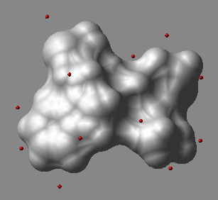
 icmMacroShape as i_complexity (8) r_gridStep (0.) r_contourLevel (1.2) l_colorByDepth (yes) l_fast (no) l_display (no) s_rainbow ("blue/white/red")

The icmMacroShape macro generates a low resolution surface

Prerequisites and arguments.

as_ : the atom/residue/molecule/object selection for which the smooth surface is built
i_complexity (8) : the number of harmonics retained in the reconstruction of the smooth density. The larger, the more detailed. The minimal complexity is 2.
r_gridStep (0.) : the step used in calculating the density and reconstruction. The zero default value means that the grid size will be adjusted automatically for large objects to avoid exceedingly large grid maps and transformations.
r_contourLevel (1.2) : the density level at which the transformed density is contoured to generate a smooth surface. The lower value will result in the larger (looser) surface envelope.
l_colorByDepth (yes) : assigns color according to the lower (than i_complexity) resolution map
l_fast (no) : uses a faster generator of the electron density, but compromises the true shape of electron density.
l_display (no) : displays the result if yes . Currently the surface is displayed as transparent solid smooth. The display can be changed from GUI using the right-click on the grob display icon or by editing the text of the macro.
s_rainbow : choose the base shape color (the first in the slash separated list), transition to the second color will highlight convex areas.

The algorithms follows these steps:

generate an electron density using a 2-exponential approximation of an atomic density ( l_fast logical allows one to activate a faster but less rigorous method ). The grid size is controlled by the first real parameter. If it is zero, the grid size is determined automatically.
perform a Fourier transformation of the electron density
truncate high frequency harmonics ( the i_complexity parameter determines the number of harmonics used in reconstruction )
generate a new electron density at lower resolution
contour this electron density at the specified level ( default 1.2 )

The surface can be further colored to highlight the depth with the occlusion shading using the color accessibility .

The output

a grob (mesh) object with a four-part name is built. The parts: "shape_" + objectName + size + complexity

icmPocketFinder macro

 icmPocketFinder as_receptorMol r_threshold ( 4.6 ) l_displayPocket (yes) l_assignSites (no)

Use this macro to find binding pocket(s) for the input as_receptorMol.

Arguments:

r_threshold: tolerance level. The lower the tolerance value the more pockets predicted and the higher the tolerance the less pockets predicted
l_displayPocket: display the first found pocket
l_assignSites: create sequence sites if you wish the site to be labeled.

The macro creates a table which contains a list of all pockets found. The table is sorted by pocket volume.

Example:

read pdb "2hiw"
convertObject a_ yes no yes yes
icmPocketFinder a_1 4.6 yes no
show POCKETS

evalSidechainFlex macro

 evalSidechainFlex rs_residues (a_) r_Temperature (600.) l_atomRmsd (yes) l_color (yes) l_bfactor (no) l_entropyBfactor (no)

evalSidechainFlex systematically samples rotamers for each residue side-chain in the input selection and uses resulting conformational ensembles to evaluate energy-weighted RMSDs for every side-chain atom. These are stored in the 'field' values on atoms and can be used for example to color the structure by side-chain flexibility. Conformational entropy for each residue side-chain is also calculated and stored in a table ATOM_FLEX

Arguments:

rs_residues: Residues evaluated
r_Temperature: Temperature used to calculated the Boltzmann distribution
l_atomRmsd: evaluate energy-weighted RMSDs for every side-chain atom.
l_entropyBfactor: the atom rmsds are normalized within the residue to reflect its total conformational entropy.
l_bfactor: the bfactors are reset to the same values that are placed in the atom 'field', and occupancy is set to be inversely proportional to it ( O=1/(1+2*rmsd) )

optimizeHbonds macro

 optimizeHbonds as  l_rotatable_hydrogens (yes) l_optimizeHisAsnGln (yes)

optimizeHbonds optimize the hydrogen bond network of the selected atom.

Arguments:

as_: atom selection for optimization
l_rotatable_hydrogens: If yes, methyl and polar hydrogen within the selection are first optimized if any water molecule is included in as_, the rotational variables of the water molecules are optimized while keeping the Oxygen fixed.
l_optimizeHisAsnGln: If yes, the optimizeHisProAsnGln macro is called to optimize the His, Pro, Asn, and Gln within the selection.

mergePdb macro

 mergePdb rs_source ( a_1.1/20:25 ) rs_graft ( a_2.1/20:25 ) s_combo ("combo")

mergePdb combines two PDB object into one and assign continuous residue number to the combined object.

Arguments:

rs_source: residue selection of the first PDB object
rs_graft: residue selection of the second PDB object
s_combo: name of the final object