
Copyright © 2026, Molsoft LLC
Mar 14 2026
Google Search:
Keyword Search:| Prev | ICM Language Reference Commands | Next |
[ add | alias | align | Append command | assign | break | build | call | center | clear | color | Color chemical | Color accessibility | Compare | compress | connect | continue | convert | copy | crypt | Date array | Delete | display | edit | elseif | endfor | endif | endmacro | Enumerate charge | Enumerate chiral | Enumerate tautomer | Enumerate library | endwhile | exit | find | fix | for | fork | fprintf | function | Global | goto | group | Gui | help | history | if | info | keep | join tables | Learn | Mlr | Learn ann | Link grob | Link group | Link variables | Link ms2ali | list | List binary | List database | list directory | list molcart | load | Macro | make | minimize | menu | modify | Modify rotate | Modify chem | montecarlo | move | pause | plot | Plot area | predict | print | Print bar | printf | print image | Query molcart | quit | randomize | read | rename | return | rotate | select | Set | show | sort | split | sprintf | store | ssearch | strip | superimpose | Superimpose minimize | Sys | test | then | transform | translate | undisplay | undisplay window | unfix | wait | web | while | write ]
ICM commands have a certain structure:
- they use command words from this list:
align assign build clear compare connect convert copy compress crypt
delete display edit enumerate exit exclude filter find fix fork fprintf group gui keep learn load
make menu minimize modify montecarlo move
pause plot predict print printf quit query randomize read redo refresh rename restore rotate
select set show sort split sprintf ssearch store strip superimpose
test transform translate undisplay undo unfix unselect unix wait write
alias antialias center color help history link list macro model sql web
accessibility alignment amber angle area aselection atom axis background ball base bar bfactor bond born boundary box catalog cavity cell chain charge cmyk column command comment comp_matrix conf cpk csd cursor chemical cistrans database distance directory disulfide dot drestraint energy error evolution factor field filename font foreground frame function gamess genome gradient grid grob hbond header html hydrogen iarray icmdb idb image index info input integer intensity inverse iupac json kernel key label library logical loop limit margin material map matrix memory merit mol mol2 moldb molcart molecule movie molsar name nucleotide object occupancy oracle origin output page parray pattern peptide pipe pdb plane postscript potential preference preview problem profile project property prosite protein pharmacophore rarray reaction real regression reflection residue resolution ring rgb ribbon regexp rainbow sarray segment selection selftether separator sequence session site size skin slide salt solution stack stdin stdout stick sstructure string surface symmetry system svariable table term tether texture topology torsion trajectory transparent tree type unknown user variable vector version view virtual volume vrestraint vselection water weight window wire xstick
add all append auto auxiliary binary bold bw cartesian clash chiral dash exact join fast fasta flat formal format full gcg gif global graphic heavy identity italic jpeg last left local mmcif mmff msf mute new none nosort number off on only pca pir pmf png pseudo pov reverse right similarity simple sln smiles smooth solid static stereo swiss targa tautomer underline unique wavefront xplor - the they arguments consisting of constants, named shell variables or expressions including functions, e.g. display ribbon Res(Sphere( a_H a_A 7.6 ))
- the order of arguments of different data type is arbitrary
- at the end of the command one may have a list of additional shell variables that will be redefined temporarily only for the duration of this command, e.g. montecarlo v_//x* mncalls=200 mncallsMC=20000 temperature=1000.
- several commands in one line can be separated by a semicolon
- commands can return certain shell variables, like i_out , i_2out, r_out , l_out , s_out , R_out , as_out .. with useful output
- to suppress command output redefine those shell variables: l_info=no or l_warn=no (for some commands there is also a mute option )
add |
[ Add column | Add matrix | Add slide | Add table ]
A family of commands adding things. Some commands use append syntax instead
It is also used as an option equivalent to append in write command.
add one or several columns or header elements to an existing table |
Adding a single column/header you may add a column (or columns) to an existing table T or create a new one if the specified name does not exist.
add column T I|R|S|P|i|r|s [name= s [append|delete] ] [index= i_pos] [mute] [local]
add header T I|R|S|P|i|r|s|M|etc [name= s [append|delete] ] [mute] [local]
(to add a row see add table args )
Adding multiple column/headers
add column T I|R|S|P|i|r|s I|R|S|P|i|r|s .. [name= S [append|delete]] [index= i_pos ] [mute] [local]
add header T I|R|S|P|i|r|s|M|etc I|R|S|P|i|r|s|M|etc .. [name= S .. ] [index= i_pos ] [mute] [local]
this command adds one or several columns to an existing table in the i_pos column (in other words if you want you column to be in the 2nd position, specify 2 as an argument). The columns are append to the end of the table by default. If the table does not exist the command will create a new table.
It an integer, string, or real are specified as an argument instead of a column-array, this value is multipled to create a column of the appropriate size.
Options:
- append: if the name option is specified prevents overwriting the column with the same name, instead modifies the provided name (e.g. 'A' -> 'A_1' )
- delete: if the name option is specified overwrites the column with the same name. Without delete (default) it will be overwritten only if the data type is the same.
- mute : The mute option suppresses the info (equivalent to temporarily setting l_info=no ).
- local : for use in macros ans shell functions: allows for local tables independent from tables with the same name at higher levels.
Examples:
add column t {1 2 3} # create a new table
add header t "A new table" name="title" # add a string to the header section
add column t {"a","b","c"} name="AA" # column AA is appended
add column t {"x","y","z"} index = 2
# adding a chemical array
add column t Parray({"CC","CC(O)=O","CCO"} smiles) name = "mol" index = 1

# adding multiple arrays
add column t {1 2 3} {3 2 1} {"a","b","c"} Parray({"CC","CC(O)=O","CCO"} smiles) name={"A","B","C","mol"}
t
 #>T t
 #>-A-----------B-----------C-----------mol--------
    1           3           a          "CC"
    2           2           b          "CC(O)=O"
    3           1           c          "CCO"
The columns can also be functions, e.g.
add column t {1. 2. 3.} {2 3 4}
add column t function="A+B" name="AplusB"
add column t function="Log(A,10)" name="log10A"
Use add column inside a macro:
macro ResAreas  rs_sel
  rs_sel = Res( rs_sel & a_*.!W )
  show surface area Mol(rs_sel) Mol(rs_sel)
  add column t Name(Res(rs_sel) full) Area(Res(rs_sel)) Area( a_1.A/A )/Area( a_1.A/A type) local name={"sel","area","rel_area"}
  set format t.sel "<!--icmscript name=\"1\"\ndisplay xstick %1\ncolor xstick cpk %1 & a_*.//c* green\ndisplay residue label %1\n\n\n--><a href=#_>%1</a>"
  if(Type(resAreas)!="unknown") delete resAreas
  rename t "resAreas"
  keep resAreas
endmacro
See also: move column , add column function
Add columns using internal functions in dynamic or static manner |
add column T function=s_expression [static] [name=s] [index= i_pos]
By default the column is added in a dynamic manner so that it can be recalculated from other columns. Option static adds the new column as a value and will not allow for the recalculation. Adds a column a string that contains an expression or a reference to one of three sources of functions:
- one of a few fast-access internal functions listed below, e.g. function="Sqrt"
- one of a thousand built-in ICM-shell functions (described in this manual), e.g. function="Icm::Min(COL)"
- an arbitrary user-defined ICM-shell function loaded from a file or ~.icm/user_startup.icm file. E.g. function="myfunc(A)"
which may contain operations with other columns in the same table. The generating expression information is attached to the column, which allows one to recalculate the values in the column using the same expression. The following functions are supported:
Basic arithmetical operations on columns are supported, examples:
add column t {1. 2. 3.} {1. 2. 3.}
add column t function="A+B" name="C"
add column t function="A-B" name="D"
add column t function="A*B" name="E"
add column t function="A/B" name="F"
add column t function="A**0.5 + B**0.5" name="G"
build column t
show t
The following mathematical and data conversion functions are supported:
Ceil, Floor, Log, Sqrt, Sign, String, PowerExamples:
add column t {1. 2. 3.} {1. 2. 3.}
add column t function="Sqrt(A)" name="C"
Chemical functionsThe following internal functions (not ICM-shell functions) are allowed in function=".." expressions (eg add column t function="MolPSA(mol)":
Examples of chemical functions usage:
add column t Chemical("CCO"//"CCCCO"//"CCCC#N")
add column t function="Nof_Atoms(mol,'*')" name="nof1"  # all atoms
add column t function="Nof_Atoms(mol,'[!H]')" name="nof2"
add column t function="Nof_Atoms(mol,'[C,O]')" name="nof3"
add column t function="Nof_Atoms(mol,'[H]')" name="nof4"
add column t function="MolWeight(mol)" name="molWeight"
add column t function="MolLogP(mol)"   name="molLogP"
add column t function="MolLogS(mol)"   name="molLogS"
add column t function="MolPSA(mol)"    name="molPSA"
add column t function="MolVolume(mol)" name="molVolume"
add column t function="MoldHf(mol)"    name="moldHf"
add column t function="calcBBBScore(mol)" index=2 name="bbbScore" append vector
add column t function="MolSynth(mol)" index=2 name="molSynth" append vector
User-defined functions
A user can defined custom function to be used in column formula expression directly : function="userFunctionName(columnArgument)"
Example:
function ligStrain( P_chem )  # returns strain for a given 3D chemical
  vwMethod = "exact"
  dielConst = 2.
  read mol P_chem name="LIGSTRAIN"
  build hydrogen
  set type charge mmff
  convert auto
  minimize cartesian "mmff" mncalls=1
  newE = Energy("ener")
  minimize cartesian "mmff" 5000
  baseE = Energy("ener")
  r_ligandStrain = newE - baseE
  delete a_
  return r_ligandStrain
endfunction

# assumes that t_3D exists and contains 3D chemicals in the mol column
add column t_3D function="ligStrain(mol)" name="strain"   # strain for every row in the table
ICM built-in shell functions.
ICM build-in functions can also be used in the expression with "Icm::" prefix.
Example:
add column drugs function = "Icm::Sum(Icm::Unique(Icm::Sort(Icm::Sarray(A.dosages.dosage:route))),',')" name="route"
Recalculating.To recalculate use the build column column_name command.
Examples:
add column T Chemical( {"c1(c(nc(N)nc1O)O)N", "c1c[nH]c2C(N=C(N)Nc12)=O"} ) name="mol"
add column T function="MolWeight(mol)" name="MW"
add T # add new row
T.mol[3] = Chemical("CC")
#
build column T.MW # recalculate mol. weights, setting the value for the new row

add column T2 {1 2 3} {4 5 6}
add column T2 function= "A+B"  # sum of two columns
See also: build column to update values, Parray ( X [ s_func ] ) to add a fixed column
Adding real arrays as matrix rows |
add matrix [ M ] R|M2
adds a matching row R or a matrix with the matching number of columns to matrix M, by stacking extra rows at the bottom. If the matrix does not exist it is created with the default name (the name is returned in s_out ) Example:
add matrix M {1. 2.} # creates new matrix M
add matrix M {3. 3.} # adds a row
show M
 #>M M
 1. 2.
 3. 3.
add matrix M Matrix(2) # adds two rows
Note that to extend the matrix horizontally (adding columns) can be done with the double-slash operator ( M1 // M2 ).
add slide to a slideshow. |
add slide [i_posInCurrentSlideshow] [s_slideTitle] [comment = s_slideComment] [ display= "-option|-option2" ]
adds a slide to the slideshow table. This table contains one parray, called slideshow.slides . If the slide position is not specified the slide will be added to the end. Alternatively, it will be inserted after the specified i_posInCurrentSlideshow
Normally the slide is saved with window layout, and graphical parameters. Those can be ignored if you add the display="-option" flag (all listed properties are 'on' by default).
- "-layout" # ignores the window/panel layout
- "-smooth" # ignores smooth view transitions between slides
- "-add" # do not overwrite the previous slide views, just add to it
- "-gf" # ignore graphical representations, inherit them
- "-color" # ignore colors , inherit them
- "-labeloffs" # do not display labels
- "-viewpoint" # ignore viewpoint changes
- "-graphopt" #
- "-mol" # do not display the chem-table window
- "-grob" # do not display grobs
- "-map" # do not display maps
- "-all" # switches off all the above properties
Example:
build string "ala ala ala"
display ribbon a_
display xstick a_/12,13 magenta
add slide "My View" comment = "Two magenta residues" display="-layout"
undisplay # hide all
# wait..
display slide "My View" # bring it back
See also: display slide , Slide
Add / insert table rows. Append tables. |
add T_1 [ i_RowNumber ] [ T_2 | row_selection | number=i_nofRows ] [ simple ]
add/insert rows (or another table with the same coloumns) to table T_1 at the target row position i_RowNumber . Use 1 (one) if you need to insert the first line. If the second table or selection is not provided, the command adds an empty row. In this case you can add number option to specify the number of rows to add/insert. The row_selection can contain rows from the same table or from a different table with a matching column structure. In the latter case, the columns may be matched by their names regardless of column order. Default values are inserted for all absent columns. The defaults for an empty line are empty string or zero value for strings or numbers, respectively. The target position will then correspond to the index of the first inserted row.
simple option toggle column matching order 'by position' instead of default 'by name'.
From version 3.6-1e the add tableName command also returns the current row as i_out .
Examples:
group table t {1 2 3} "a" {"b","d","e"} "b"
show t
 #>T t
 #>-a-----------b----------
    1           b
    2           d
    3           e

add t 1 # insert empty line before 1st
show t
 #>T t
 #>-a-----------b----------
    0           ""
    1           b
    2           d
    3           e

group table t {1 2 3} "a" {"b","d","e"} "b" # recreate the table
add t 3 t[1]  # insert a duplicate of 1st row after the 2nd
show t
 #>T t
 #>-a-----------b----------
    1           b
    2           d
    1           b
    3           e

group table t {1 2 3}  "a"  {"b","d","e"} "b"  # recreate the table
group table tt {1 2 3} "c" {"b","d","e"} "b" {4 5 6} "a" # another table
# order is diffferent, extra column present
add t 3 tt[1:2]  # or add t 3 tt.aa<3
show t
 #>T t
 #>-a-----------b----------
    1           b
    2           d
    4           b
    5           d
    3           e
alias |
alias abbreviation word1 word2 ...
create alias
alias delete abbreviation
delete alias
It is important that the abbreviation is not used in the ICM-shell. The same names can not be given later to ICM-shell objects.
Alias may contain arguments $0, $1, $2, etc. ICM-shell will pick space-separated words following the alias name and substitute $1, $2, etc. arguments by the specified argument. $0 stands for all the arguments after the alias name.
Examples:
 alias seq sequence                    # seq will invoke sequence
 alias delete seq                      # delete alias name seq
 alias dsb display a_//ca,c,n          # abbreviate several words to
                                       # reduce typing efforts
                                       # aliases with arguments
 alias NORM ($1-Mean($1))/Rmsd($1)
 show NORM {6,7,8,4,6,5,6,7,5,6}       # make sure there is no space
align |
[ Align number chemical | Align res numbers | Align sequence | Align fragments | Align 3D | Align 3D heavy ]
align number chemical: canonically rename atoms in hetero molecules |
align number chemical ms_het_molecules
Examples:
read pdb "3gvu"
align number chemical a_H.  # rename atoms in both ligands
align number: renumber residues sequentially |
align number rs_residuesToBeRenumbered i_first|s|I|S [molecule]
align number ms_chainsToBeRenumbered [ i_firstNumber ]
renumber selected residues, or residues in selected molecules or objects sequentially in all of them from starting one or the specified first number. May be useful to deal with messy numbering in some pdb-files. Option molecule will start numbers from 1 or i_first in each molecule. Chain ids are also allowed, e.g. set number a_/13 "13A". Multiple residues can be set with integer or string arrays of labels. If integer array contains the same numbers, e.g. 10,10,10 the labels will get the insertion characters, e.g. 10,10A,10B .
Examples:
 read pdb "1crn"
 align number a_1            # renumber all res. 1 to N
 align number a_1/10:20 101  # just the selected residues from 101
 align number a_1       101  # renumber all res. 101 to 100+N
 read pdb "2ins"
 align number a_/* 1
 align number a_/* 1 molecule # each chain starts from 1
align number ms_chainsToBeRenumbered seq_master [ i_offset ] renumber the residues of the selected molecule according to seq_master master sequence which is aligned to the sequence of the selected chain. The alignment (pairwise or multiple) need to be linked to the molecule/chain and both the chain sequence and the master sequence need to be covered by the alignment. The molecular sequence can be generated with the make sequence [ ms_chainsToBeRenumbered ] command.
This command may be useful in cases in which a structural model does not represent the entire sequence because of omitted loops, N- and C- termini, while you still want to keep the numbering according to the full master sequence. You might want to use the command also on models by homology generated with the build model command.
Example:
 seqmaster = Sequence("ACDEFGHIKLMNPQRST")
 build string   "DEFGH-----PQRST"  # dashes are skipped
 make sequence a_1 name="seqmodel"   # sequence is auto-linked
 a = Align(seqmodel,seqmaster)       # linked alignment
 align number a_1 seqmaster
 # Info> residues of a_def.m renumbered by sequence 'seqmaster' from alignment 'a'
 display residue label
align: ICM multiple alignment algorithm |
align ali_SequenceGroupName [ tree=|filename= s_epsFileName ]
align sequence [selection] | seq1 seq2 .. | seedSequence [ min_seqID (20.)] [ name=s ]
make a multiple alignment of specified sequences.
The sequence group may result from the group sequence s_groupName command.
The input arguments include the following:
- seq1 seq2 ... : explicitly specified
- sequence : all sequences in the shell
- sequence selection : all sequences selected in GUI
- seqGroup : sequences grouped together previously
- seedSequence : sequences in the shell similar to the specified with optional min_seqID (default 20%).
For pairwise alignment use the Align( seq1 seq2 ) function. The algorithm includes the following steps (inspired by corridor discussions with Des Higgins, Toby Gibson and Julie Thompson ):
- align all sequence pairs with the ICM ZEGA algorithm, and calculate pairwise distances between each pair of aligned sequence with the Dayhoff formula, e.g. the distance between two identical sequences will be 0. , while the distance between two 30% different sequences will be around 0.5. The distance goes to an arbitrary number of 10. for completely unrelated sequences. The distance matrix Dij can later be extracted from the alignment with the Distance( ali_ ) function.
- build an evolutionary tree from Dij with the "neighbor-joining algorithm" of Saitou, N., Nei, M. (1987) to determine the order of the alignment and calculate relative weights of sequences and profiles from the branch lengths. The tree will be saved in the file defined by the tree= s or filename= s option . Starting from version 3.5-2 the aligTree.eps file is NO LONGER saved by default). The so-called Newick tree description string will be saved in s_out .
- traverse the tree from top to bottom, aligning the closest sequences, sequence and profile or two profiles. After each Needleman and Wunsch alignment, build the profile.
- generate the final neighbor-joining evolutionary tree and write the PostScript file with the tree to disk.
Examples:
   read sequences s_icmhome+"zincFing"
   list sequences               # see them, then ...
   group sequence alZnFing      # group them, then ...
   align alZnFing               # align them
   align alZnFing filename="znTree.eps"  # eps file with a tree
  read sequence swiss web "12S1_ARATH"
  read sequence swiss web "12S2_ARATH"
  group sequence arath
  align arath
EST,DNA alignment and assembly |
[ sim4 ]
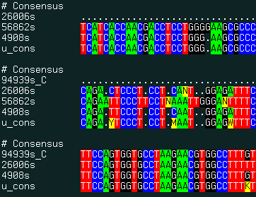
align new ali_sequenceGroup [ seq_seed ]multiple alignment of ESTs and genomic DNA and consensus derivation. This command uses the external the sim4 program to generate pairwise alignments between expressed DNA sequence and a genomic sequence. The program can be downloaded from the http://globin.cse.psu.edu/globin/html/docs/sim4.html site.
The procedure has the following steps:
The result of this command is best displayed with the show color ali_ command. |
|
An example:
 read sequence "http://www.ncbi.nlm.nih.gov/UniGene/" + \
     "download.cgi?ID=5198&ORG=HsLINE=1" #
 read sequence "../Hs5198"
 group sequence unique u # squeeze out obvious redundancies and form group 'u'
 align new u             # form multiple alignment and build consensus
 show color u
See also:
- filtering, group sequence unique=".."
- Trans ()
- show [color] ali_
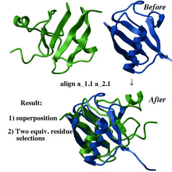
align two molecules by their backbone topology |
align [ distance ] ms_1 ms_2 [ i_windowSize (15) ] [ r_seqWeight (0.5) ]
| This command finds the residue alignment (or residue-to-residue correspondence) for two arbitrary molecules having superposable parts of the backbone conformations. The structural alignment identification and optimal superposition is primarily based on the C-alpha-atom coordinates, but the sequence information can be added with a certain weight (the default value of r_seqWeight is 0.5 which was found optimal on a benchmark). The structural alignment algorithm is based on the ZEGA (zero-end-gap-alignment) dynamic programming procedure in which substitution scores for each i,j-pair of residues contain two terms: |
|
- structural similarity in a i_windowSize window between two fragments surrounding residues i and j, respectively. This similarity is calculated as local Rmsd of the residue label atoms (these atoms are C-alpha atoms by default but can be reset to other atoms with the set label command, e.g. set label a_*.//cb ). If the option distance is specified the deviation of the interatomic distances between equivalent pairs of atoms (so called distance rmsd ) is calculated instead of a more traditional root-mean square deviation between atom coordinates of equivalent atoms. The latter method is less accurate but an order of magnitude faster.
- sequence similarity (if r_seqWeight > 0.). Average local sequence alignment score in the i_windowSize window is calculated for i,j-centered pair of fragments. In this sense this sequence similarity is different from the one used in pure sequence alignment (see the Align function), in which just the i,j residue pair is evaluated. The default value of r_seqWeight of 0.5 is rather mild (about a half of the structural signal).
The output:
- ali_out contains structural alignment (if sequences linked to the molecules do not exist, they will be created on the fly). The alignment can be further edited with the interactive alignment alignment editor.
- as_out contains the residue selection of the aligned residues in the first molecule
- as2_out contains the residue selection of the aligned residues in the second molecule
- M_out , the matrix of local structural/sequence similarity in a window is retained and can be visualized by:
- r_2out the result RMSD
Example:
read pdb "1ql6"
read pdb "2phk"
align a_1ql6. a_2phk.
make grob color 10.*M_out name="g_mat # x,y,z scales
display g_mat
# or
plot area M_out display grid link
See also:
- Align( seq_1 seq_2 distance|superimpose ). This function creates the first unrefined structural alignment as described above.
- find alignment which refines initial structural alignment.
  a = Align(... superimpose )  # superposition/RMSD based local str. alignment
  a = Align(... distance    )  # distance RMSD based local str. alignment

  find a superimpose 4.0 0.5
Example:
  read pdb "1brl"
  read pdb "1nfp"
  rm a_*.!A
  display a_*.//ca,c,n
  color molecule a_*.
  align a_2.1 a_1.1
  center
  show String(as_out) String(as2_out)
  color red as_out
  color blue as2_out
  show ali_out
align heavy command for multiple alternative structural alignments. |
align heavy rs_1 rs_2 [ r_rmsd ] [ i_windowSize [ i_minFragment]] [ r_elongationWeight]
This method, as opposed to the default align ms_1 ms_2 generates many possible solutions and does not depend on sequential order of the secondary structure elements. However, it leads to a combinatorial explosion and is intrinsically less stable computationally, and generally requires more time. The command finds the optimal 3D superposition between two arbitrary molecules/fragments (two residue selections rs_1 and rs_2 ).
The procedure generates structural fragments of certain initial length and superimposes all of them to calculate the structural similarity distance. Then the "islands" of similarity are merged into larger pieces. This process is controlled by the following arguments: i_windowSize is the residue length of structural fragments for the initial fragment superposition. Fragment pairs with the rms deviation less than r_rmsd are then combined, giving composite solutions of total residue length larger than i_minFragment. Acceptance or rejection of the composite solutions is governed by the following score (the smaller, the better)
score = rmsd - (1.37 + Sqrt(1.16 * length - 15.1)), length >= 14
If length > 14 , we use linear extrapolation of the score dependence:
score = rmsd - (1.37 + 1.068*(length-13))
The score is required to be less than r_rmsd. Practically, for longer fragments one can find much larger RMS deviations according to the length correction of the score.
Defaults:
- r_rmsd = 1. A
- i_windowSize = 15 residues
- i_minFragment = i_windowSize
- r_elongationWeight=0.1
See also: How to optimally superimpose without the residue alignment
Example:
read pdb "4fxc" read pdb "1ubq" display a_*.//ca,c,n color molecule a_*. align heavy a_1.1 a_2.1 12 1.5 .1 center load solution 2 # load the second best solution color red as_out color blue as2_out for i=1,10 load solution i color molecule a_*. color red as_out color blue as2_out pause # rotate and hit 'return' endforNote. Increase i_minFragment parameter (12 in the above example) to something like 20 if the program hangs for too long. Interrupt execution with the ICM-interrupt (Ctrl \) if you want only the top solutions.
append (commands) |
[ Append sequence | Append stack | Append column ]
There is a family of commands starting with the append keyword. They are usually used to add sub-elements to a compound object like an alignment or a stack. In many cases ICM uses add syntax instead of append.
Appending sequences to a sequence group or an alignment |
append ali_seqGroup seq_1 seq_2 .. .
appends sequences to a sequence group. This may be required if you formed a sequence group for future alignment or filtering/compression and you want to append additional sequences to it.
Examples:
read sequence group "bunch.seq" name="xx" # group xx is formed
append xx my_seq  # appending your sequence to xx
group xx unique   # filter out identical ones
align xx
read sequence swiss web "12S1_ARATH"
read sequence swiss web "12S2_ARATH"
group sequence name="arath"
read sequence swiss web "14310_ARATH"
append arath 14310_ARATH
align arath
Appending a molecule or a ligand stack to an existing stack |
append stack s_ligandStackFileName [i_maxConf]
append stack os_ligandObject
this command takes a stack which corresponds to a receptor object and appends each conformation in the stack with a conformation of the ligand. If the ligand conformation can be taken from either from a stack file, this command will combine each conf from the main stack with all conformations from the file. The i_maxConf argument will set the limit on how many conformations are taken from the ligand stack (i.e. append stack "lig.cnf" 1 will combine only the first conformation of the ligand )
If the second argument is an ICM object, each conf of the current stack will be extended with the variables from the ligand. Now the ligand object can be appended to the receptor object with the move command and the new combined object can use the expanded stack.
build string "ACDEF"  # the "ligand" peptide
rename a_ "Lig"
translate a_ {10. 0. 0.} # shift not to overlap with a_Rec.
montecarlo v_//!?vt*     # created Lig.cnf stack

build string "RSTVW"  # the "receptor" peptide
rename a_ "Rec"
montecarlo v_//!?vt*     # created Rec.cnf stack

move a_1. a_2.    # ligand must be the 1st argument
append stack "Lig.cnf" 4 # combine up to 4 best ligand confs
minimize stack    # minimizes each stack conf
load conf 1       # check them out
append two tables via two columns with matching values |
append t1.A t2.B
Append rows of table t2 to table t1 by rows corresponding to unique column t2.B . The t1.A column values do not need to be unique.
group table people {"J","C","M"} "p" {"MS","MS","MS"} "orgid"
group table orgs  {"MS"} "id" {"Molsoft"} "name"
append people.orgid orgs.id
people
 #>T people
 #>-p-----------orgid-------name-------
    J           MS          Molsoft
    C           MS          Molsoft
    M           MS          Molsoft
This command is a particular case of a more general join command.
See also the add table command for adding rows from a column with identical column structure (e.g.
add t tt ).
assign |
[ Assign sstructure | assign sstructure segment ]
assign sstructure: derive secondary structure from a pattern of hydrogen bonds |
assign sstructure rs [{ s_SecondaryStructTypeCharacter | s_SSstring }]
Manual assignment of a desired secondary structure annotation to a residue fragment
assign sstructure rs { s_SecondaryStructTypeCharacter | s_SSstring }
assign specified secondary structure to the selected residues rs_ , e.g.
 read pdb "1crn"
 assign sstructure a_/* "_"  # make everything look like a coil
 cool a_
 assign sstructure a_/1:10 "HHHH_EEEEE"
 cool a_
|
This command does not change the geometry of the model, it only formally assigns secondary structure symbols to residues. Note: to change the conformation of the selected residue fragment, according to a desired secondary string, use the ICM -object and the set command applied to both sequences and molecular objects. |
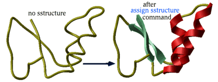
Automated derivation and assignment of secondary structure from atomic coordinates
assign sstructure rs
If the secondary structure string is not specified, apply ICM modification of the DSSP algorithm of automatic secondary structure assignment (Kabsch and Sander, 1983) based on the observed pattern of hydrogen bonds in a three dimensional structure.
The DSSP algorithm in its original form overassigns the helical regions. For example, in the structure of T4 lysozyme (PDB code 103l ) DSSP assigns to one helix the whole region a_/93:112 which actually consists of two helices a_/93:105 and a_/108:112 forming a sharp angle of 64 degrees. ICM employs a modified algorithm which patches the above problem of the original DSSP algorithm. Assigned secondary structure types are the following: "H" - alpha helix, "G" - 3/10 helix, "I" - pi helix, "E" - beta strand, "B" - beta-bridge, "_" or "C" - coil.
Examples:
 nice "1est"       # notice that many loops look like beta-strands
 assign sstructure # now the problem is fixed
 cool a_
See the set rs_ s_SecStructPattern command to actually set new phi, psi angles to a peptide backbone according to the string of secondary structure.
assign sstructure segment |
assign sstructure segment [ ms_molecules ] # ms_ICMmoleculesPreferable
create simplified description of protein topology (referred to as segment
representation). Segments shorter than segMinLength are ignored.
The current object is the default.
This command will work both on un converted pdb files as well as the pdb files.
However the resulting secondary structure will be BETTER when the structure is converted and
hydrogens are added.
See also
show segment,
ribbonStyle,
display ribbon.
convert
convertObject
break |
[ assign residue ]
is one of the ICM flow control statements. It permits a loop ( e.g. for or while ) to be broken before calculations have completed.Examples:
   for i = 1, 8
     print "Now i = ", i, "and it goes up"
     if (i == 4) then
       print "... but at i=4 it breaks, Ouch!"
       break
     endif
  endfor
See also
goto .
assign residue |
Assigns residue structure to a peptide or a protein. Sometimes when you read a peptide or protein from MOL or MOL2 with no residue information present it is treated as a single residue small molecule. This command allows to restore residue layer.
assign residue os1
Example:
build string "EACARVAAACEAAARQ"
read mol Chemical( a_ exact hydrogen )  name="xxx"  # read it as a single residue small molecule
assign residue a_   # restore residue structure
Sequence( a_1. )
Sequence( a_2. )
build |
[ Build atom | Build column | Build conf | Build sequence | Build string | build tautomer | Build model | Build loop | Build smiles | Build hydrogen | Build molcart ]
The build family of functions allows one to create molecular objects- from sequence file ( build s_seqfile )
- from sequence string ( build string)
- from a linear chemical notation ( build smiles )
- from a sequence and a template by homology ( build model )
build one atom and rebuild hydrogens |
build atom as1 [simple] [s_elementName=("c")] [i_bondType=(1)]
build pseudo as_inICMobj
by default it will add a carbon to the selected atom in a non-ICM object
and rebuild hydrogens for the affected atoms.
Use the strip command for ICM objects.
Options and arguments:
- simple does not rebuild hydrogens.
- s_elementName is a string with the name of the chemical element.
- i_bondType is 1 for a single bond (the default), 2 for a double bond and 4 for a triple bond.
Example:
build smiles "CC(C)Cc1ccc(cc1)C(C)C([O-])=O" name="ibuprofen"
strip a_ibuprofen.
build atom a_ibuprofen.m//c1 "n"
build atom a_ibuprofen.m//c1 2
See also:
Recalculating dependent columns |
build column T.col|T
Rebuilds all values in a dependent column T.col
build column T | T_row_selection
Rebuilds all dependent columns in the table T_ or row selection (e.g. T[12], or T.ID==123 ) If column A depends on column B and column B depends on other columns, column B will be calculated before column A.
Examples:
add column T {2 5 1} name="B"
add column T function="A + B" name="C"
add column T function="C + B" index=1 name="D"
T.A[1] = 10
build column T[1] # should change values of C and D in the first row
See also: add column function
Generating low energy conformations for small molecules. |
build conf T.mol # requires GINGER license
Building object from sequence file |
build s_IcmSeqFileName [name=s_objName] [ library= { s_libFile | S_libFiles} ] [ delete ]
build string s_IcmSeqString [name=s_objName] [ delete ]
(a more flexible way to get a sequence you want, see build string for more details)
reads s_IcmSeqFileName.se
ICM-sequence file and builds an ICM molecular object.
This sequence file is different from a simple sequence file and contains three
(sometimes four) character residue names defined in the
icm.res residue library file (try show residue types to see the list).
Use command build string if you want to build an object from a string with one letter coded sequences or a named sequence. E.g. build string "ASDGF" or "ASD;DERR" or "nh2 ala his cooh"
To get a D-amino acid instead of L-ones simply
use D as a prefix: Dala Darg. Specify N- or C-terminal modifiers directly
in the file if needed. The build command will create them in some default
conformation (extended backbone with different molecules oriented around
the origin as a bunch of flowers). Several molecules can be specified in
the ICM sequence file.
Residue names may contain numbers (i.e. 4me ). However, the residue numbers
with a modification character, such as 44a, 44b should contain a
slash before the modification character (i.e. 44/a , 44/b ). An example
in which we create a sequence of residues ala and 4me with numbers 2a and 2b,
respectively: "se 2a ala 2b 4me".
The library option lets to temporarily switch the library file. The same result may
also be achieved by redefining the LIBRARY.res array of the LIBRARY table.
The delete option temporarily sets the l_confirm flag to no
and the old object with the same name gets overwritten.
Examples:
 build "def"  # def.se file
 build s_icmhome + "alpha.se"  # alpha.se file
 build "wierd" library="mod.res"  # get residues from mod.res
#
 LIBRARY.res = {"icm","./myres"}
 build "s"
Building object from string |
build string s_IcmSequence [ name= s_ObjName ] [ delete ] [i_first_amino_residue_number (1)]
create an ICM-object from a s_IcmSequence string (see the build command above). To get a D-amino acid instead of L-ones simply use D as a prefix: Dala Darg. Specify N- or C-terminal modifiers directly in the file if needed. The build command will create them in some default conformation.
The build string command also understands short one line version of the full format. The short format looks like "ASD" or "ala his" and may not start from "ml " or "se ".
The possibilities are the following:
- one letter code, - it needs to be specified in upper case letters, e.g. "DD";
- full three-four letter code, e.gg. "nter ala hise Dala cooh"
- multiple molecules - just use a comma, a semicolon or a dot as a separator, e.g. "WWWW;AAAA;EEE" or "ala his trp; nh3+ gly coo-"
- mixed one-letter and three letter code, e.g. "AST-sep-tpo-AAA" to include phosphoserine and phosphothreonine
If the sequence is provided as one letter code (e.g. "ACDTCAA") or as an icm sequence the residue number of the first aminoacid will be set to 1 unless redefined by the optional integer i_first_amino_residue_number.The N-terminal residue "nh3+" will then get number 0.
Option delete temporarily sets the l_confirm flag to no
and the old object with the same name gets overwritten.
Examples:
   build string "ADG-sep-HRTE" # the charged terminal groups will be added, note phosphoserine
   build string "ADGHRTE" 2 # assign res number of 2 to 1st alanine
   build string "ADGH;RTE" # two peptides, a and b
   build string "nter ala Dhis cooh" name="pep"  # one peptide named a_pep.
   build string "ml a \nse nh3+ his coo- \nml b \nse trp" # molecules a and b
   build string IcmSequence("GHFDSFSDRT","nter","cooh") # translate and add termini
#
# Using alias  BS   build string "se $0"
   BS ala his trp
See also: build sequence, Sequence, IcmSequence.
build tautomer |
build tautomer [charge={r_pH,r_window}] ms_het|rs_tautomeric_residues"
prepares internal data for quick switching between different tautomer states of small molecules ms or histidine rs_his by relative tautomer number or histidine tautomer name.
charge option adds enumeration of format charge states at given pH and a window.
You need to call this command if you plan to sample different tautomers in montecarlo command (~~tautomer option)
Example:
build string "AHW"
build tautomer a_/his # adds a hydrogen and hydrogen masks to allow the switching
monecarlo reverse tautomer
Example:
 build smiles "C(CNN)c1ccccc1"
 build tautomer a_1 charge = {7. 2.}
 set tautomer a_1 1
 set tautomer a_1 2
 set tautomer a_1 3
See also: set tautomer enumerate charge
Building model by homology |
[ Homology steps | Loop search | The output ]
build model seq_1 seq_2 ... ms_Templates ... [ ali_1 ...] [ margin= { i_maxLoopLength, i_maxNterm, i_maxCterm, i_expandGaps }build a comparative model (homology model) of the input sequences based on the similarity to the given molecular objects. The margin arguments:
| name | default | description |
|---|---|---|
| i_maxLoopLength | 999 | longer loops are dropped |
| i_maxNterm | 1 | the maximal length of the N-terminal model sequence which extends beyond the template |
| i_maxCterm | 1 | the maximal length of the C-terminal model sequence which extends beyond the template |
| i_expandGaps | 1 | additional widening of the gaps in the alignment. End gaps are not expanded |
-
Possible modes:
- simple one-to-one mode: build model seq_1 [ms_1] [ali_1]
- N sequences - N corresponding molecules: build model seq_1 seq_2 .. seq_N ms_1,2,..N This mode requires the minimize tether command to complete the construction.
Examples:
 l_autoLink = yes
 read pdb "x"
 read alignment "sx"
 build model ly6 a_
 ribbonColorStyle = "alignment" # grey-gaps, magenta-insertions
 display ribbon
 read pdb "2ins"  # multichain
 a = Sequence( "GIVEQCCASV CSLYQLENYC N" )
 b = Sequence( "VNQHLCGSHL VEALYLVCGE RGFFYTPKA" )
 c = a
 d = b
 build model  a b c d a_1.
 minimize v_//V "tz" 1000
# or   minimize tether
# Now optimize the side chains
 selectMinGrad = 1.5
 set vrestraint a_/*
 montecarlo fast v_/!I/x*
# !It means residues which are not Identical to their template residues
# use  refineModel to energetically optimize the model
The algorithm performs the following steps: |
Alignment adjustment: modifies the alignment according to i_expandGaps, and prepare a sequence with the ends and the long loops truncated according to the alignment and the { i_maxLoopLength , i_maxNterm , i_maxCterm } parameters.
Building a straight polypeptide from the model sequence: builds a full-atom polypeptide chain for this new sequence. The residues in your model are numbered according to the template and all the inserted loops residues are indexed with 'a','b', etc. E.g. the numbering may look like this: 200,201,203,204,204a,204b,204c,205 ... This numbering allows one to follow more easily the correspondence between the template and the model. If you do not like this numbering scheme, just use the
align number a_/*command and the model residues will be renumbered from 1 to the number of residues.
Backbone topology transfer: inherits the backbone conformation from the aligned (but not necessarily identical) parts of the known template
Identical side-chain building: inherits conformations of sidechains identical to their template in the alignment
Non-identical side-chain placement: assigns the most likely rotamer to the side chains not identical in alignment. If you want to do more than that apply:
set vrestraint a_/*  # assigns the rotamer probabilities
montecarlo fast v_/Cx/x* # x* selects for all chi (xi) angles
You can also manually re-optimize any side chains either interactively (right-mouse click on a residue atom, then select Shake Amino-Acid Side-Chain) or from a script, e.g. for residue 14:
set vrestraint a_/*  # assigns the rotamer probabilities
montecarlo v_/14/x*
ssearch v_/14/x*     # systematic conformational search for the 14-th sidechain
Loop searches: |
searches the icm.lps which may contain entire PDB-database for suitable loops with matching loop ends and as close loop sequence as possible, inserts them into the model and modifies the side-chains according to the model sequence.
The loop file can be easily customized, updated and rebuilt with the write model [append] command in a loop over protein structures. To use your custom loop file, redefine the LIBRARY.lps variable. The loops can be loaded into a fragment of a protein or peptide with the build loop stack rs_loop command (eg build loop stack a_/3:15 ).
Loop refinement and storing alternatives: adjusts the best loops found and keeps a stack of loop alternatives which can later be tested (see the Homology gui-menu).
The output |
The build model command returns the following variables:
LoopTable master table containing list of all the loops, their conformation in alphanumeric code, a measure of the deviation of the database loop ends and the model attachment sites, the loop length and the numerical conformation type (not really important). E.g.
#>T LoopTable
#>-1_Loop------2_Conf------3_Rmsd------4_Nof-------5_Type-----
   a_ly6.a/7:10 31R21       0.1         11          1
   a_ly6.a/60:63 1RRR32      0.1         8           1
   a_ly6.a/43:46 211331RRRR  0.240658    4           1
Individual loop tables
Tables called LOOP1 , LOOP2 , etc. for each inserted loop. The tables contain the coded conformational string, relative energy, the position of the offset in the structure database file ( offset ) to be able to extract this loop again, and the rmsd of the loop ends. Example:
icm/ly6> LOOP1
#>T LOOP1
#>-Conf--------energy------offset------rmsd-------
   31R21       0.          3623594     0.092104
   31RR2       1.519275    3427772     0.083372
   R1121       1.612712    3750108     0.097777
   R1R32       1.639177    1529882     0.087113
   R1RR2       1.880638    3806768     0.079335
   31R32       3.714823    4561270     0.053853
   R3RR2       4.531406    4003324     0.042881
Writing and restoring the tethers Objects, alignments and tethers can be written to a single binary project file (see write binary all ), for example
write binary object tether sequence alignment "/tmp/tmp.icb"
Trouble shooting build model may crash. A possible reason of the crash is that the pdb file is not correctly parsed due to formatting errors. Many pdb files still have formatting errors, especially those which are generated by other programs or prepared manually. In this case the read pdb command is trying to interpret the field shifts and, as with any guess work, frequently gets it wrong. For example, try 2ins and you will see that the atom or residue names are shifted. To fix the problem, try to use the exact option of the read pdb command.
Building loop to a model by homology |
build loop [stack] rs_fragments
rebuild specified loop based in a PDB-database search (see build model ).
An example:
 read object s_icmhome+"crn"
 build loop a_/20:26  # rebuild this loop
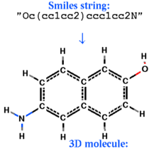
Building object from a chemical smiles string |
build smiles s_smiles_string [ name= s_ObjName]
|
create an ICM-object from the smiles -string, respectively. Set l_readMolArom to no if you do not want to assign aromatic rings from a pattern of single and double bonds (and formal charge and bond symmetrization for CO2, SO2, NO2or3, PO3 ) upon building. To suppress the symmetrization and consequential charging of CO2, set the l_neutralAcids flag to yes . |
Examples:
build smiles "CCO"   # ethanol

build smiles "Oc(cc1cc2)ccc1cc2N"

build smiles "Oc(cc1cc2)cc(ccc3)c1c3c2"

build smiles "C/C=C\C" # cis-2-butene

build smiles "C/C=C/C" # trans-2-butene

              # dicoronene
build smiles "c1c2ccc3ccc4c5c6c(ccc7c6c(c2c35)c2c1c1c3c5c6c"+\
             "(c1)ccc1c6c6c(cc1)ccc1ccc(c5c61)cc3c2c7)cc4"

              # NAD
build smiles "[O-]P(=O)(OCC1OC(C(O)C1O)N1C=2N=CN=C(N)C=2N=C1)"+\
             "OP(=O)([O-])OCC1OC(C(O)C1O)N=1C=CC=C(C=1)C(=O)N"

              # Hexabenzo(bc,ef,hi,kl,no,qr)coronene
build smiles "c1c2c3c4c(ccc3)c3c5c(c6c7c(ccc6)c6c8c(ccc6)c6c9"+\
             "c(ccc6)c(cc1)c2c1c9c8c7c5c41)ccc3"

              # rubrene
build smiles "c1c2c(c3ccccc3)c3c(c(c4ccccc4)c4c(cccc4)c3c3ccccc3)"+\
             "c(c2ccc1)c1ccccc1" name="rubrene"
Sometimes the build smiles command is not sufficient. The molecule needs
to be optimized in the mmff force field and several conformations
need to be sampled.
A more rigorous conversion is provided by the convert2Dto3D macro.
See also: Smiles , find molecule.
Building hydrogens according to topology and formal charges. |
build hydrogen [ as_heavyAtoms ] [ i_forcedNofHydrogens ] [cartesian]
adds hydrogens to the specified heavy atoms according to their type and formal charge. All heavy atoms of the current object are used by default. If your have hydrogens already and their configuration is wrong, you can delete them with the delete hydrogen command. The number of hydrogens may be enforced if the optional i_forcedNofHydrogens argument is specified.
Option cartesian means that no new hydrogens are added, but, rather, the existing ones are set to new coordinates according to the heavy atoms (a better syntax for this action is set hydrogen ).
See also the set bond type command, set hydrogen .
Examples:
  read mol s_icmhome+ "ex_mol"  # several small molecules
  display a_4.
  build hydrogen a_4.  # added and displayed
#
  undisplay
  display a_3.
  build hydrogen a_3.
# move one of the nydrogens
  build hydrogen a_3. cartesian # should put the hydrogen back at a correct position
Building molcart indices for substructure, similarity or exact search |
build molcart {s_tableName|S_tableNames} [sstructure|similarity|exact]
builds (or rebuilds) various keys for molcart table.
call |
call s_ScriptFileName [ only ]
invokes and executes an ICM-script file. End the script with the quit command, unless you want to continue to work interactively, or use it in other script.
The option only allows one to suppress opening the script file if the call command is inside a block which is not executed. By default the script file is opened and loaded into the ICM history stack anyway, but the commands from the file are not executed.
The absolute path of the script can be obtained by calling the Path ( last ) function.
Example:
  call _startup             # execute commands from _startup file
  show Path( last )
Example of calling scripts inside conditional expressions.
if Type( CONSENSUS ) != "table" then
 call _startup only # only means do not read if the table is already loaded
endif
center |
center [ { as | grob } ] [ only ] [ static | plane ] [ margin= r_margin ]
centers and zooms the screen on selected atoms as_ or graphics objects. Default objects: all existing atoms and graphics objects. The r_margin argument is given in Angstrom units and can be used to set a relative size of the selection and the frame. Normally all dimensions of the molecule/grob are taken into account, so that the molecule can be rotated without changing scale.
Options:
- only : do not rescale, translate only, i.e. move the selected atoms to the center of the graphics window
- static : scale only according to the visible X-Y dimensions and the margin. Do not take the Z-dimension into account in the size calculation as if you do not intend to rotate objects. That implies an assumption that the orientation of molecules/grobs/maps will not be changed.
- plane : center plane uses GRAPHICS.clippingPlane parameter and has additional options, see below
Examples:
   nice "1est"
   center
   center Sphere ( a_/15:18 )
   center a_/1:2 only  # keep the scale

   read grob s_icmhome+"beethoven" # a genius
   display beethoven smooth
   center beethoven static   # 10 A margin
center plane foreground|background
command to set clipping planes by resetting four compounds of the GRAPHICS.clippingPlane variable. Make sure to set GRAPHICS.clipStatic to yes.
clear |
[ clear-error ]
clear
clear terminal screen
clear selection
clear the graphical selection as_graph
Example:
nice "1crn"
as_graph = a_/1:5 # select five residues
clear selection # nothing again
clear pattern chemarray
clear SMARTS search attributes in the input chemical array.
Example:
add column t Chemical("[C;D2]")
clear pattern t.mol   # D2 attribute will be cleared
See also: Exist pattern
clear graphic [ os ]
clears display properties , graphic representation memory and reset the graphic planes to the default.
clear error
clears all error and warning bits previously set by ICM. See also Error ( i_code )
color |
[ Color specification | Color object ]
The color command colors different shell objects, their parts, or different graphical representations with by colors specified in various ways. The main color commands are listed below:color all|{wire|xstick|cpk|surface|skin|[residue|atom|variable|string] label|ribbon [base]} color as [full]
color as|rs|ms {molecule|object|alignment | R_values [window=R2_fromTo] } [full] [all]
color background|volume color # volume for the depthcuing fog color
color chemical X_chemarray {P_predictiveModel | pharmacophore }
color site ms1 index=i_site|I_sites color_spec
color distance|hbond|angle|torsion P_distParray color
color g accessibility r_depth ([0:1]) # occlusion coloring
color g [add|pseudo] color as GROB.atomColorRadius= r
color g map [m_valuesForColoringGrob]
color g|grob potential [ fast ] [ reverse | simple ] [ms_sourceAtoms] # electrostatic coloring
color map_Name [ I_colorTransferFunction ] [ R2_fromTo ] [ auto ]
Options:
- full : allows one to set colors for atoms that are not displayed in addition to the displayed ones. The default only changes colors of the atoms visible in a given representation. (this option has been added in versions compiled after Sep 15, 2009). This option replaces the set color command for batch coloring.
- all : colors all graphical representations (by default it colors only the specified ones)
To change some of the color defaults permanently edit icm.clr file or these preferences (you may change preferences via GUI or directly in session or user_startup ):
See also: set color to set atom or residue color directly and without graphics.
See also: icm.clr for allowed color names and their r,g,b values;
the plot command needs ICM colors , an sarray can be returned with the Color( R ) command.
Specifying colors in ICM |
There are various ways to specify a color in ICM: by name, index or RGB representation.
color_name | color[i_index] | i_Color | r_Color | rgb=rgb_color
Specifying color by name:
color redOther color name examples: black, white, grey, blue, red, yellow, green, orange, magenta, lightblue. Color names may be observed and changed in the icm.clr file.
Requesting contrasting colors by index:
color color[4]This call uses color number 4 from the list of "named" colors (first section of the icm.clr file). Colors with their numbers can be listed by the show color command and their total number is accessible via the Nof( color) function. This mode is useful if you need to color selected elements with contrasting colors rather than with a smooth spectrum.
Example:
  read pdb "1crn"
  display ribbon a_1crn.
  show colors
  color a_/1:5/* color[89]
  for i=1,Nof(a_/*)
    color a_/$i color[i]       # speckled coloring
  endfor
Specifying color by index:
color 3
Color indices are taken from the "rainbow" section of the icm.clr file. Currently there are 128 colors (i=0,127) in this section and they form a smooth transition from blue to red via white (not really a rainbow). You may change the "rainbow" colors in the icm.clr file. Number 128 becomes blue again. Using integer color indices is convenient for automatic coloring within ICM loops.
Example:
   display "Colors"
   for i=1,255
     color background i
     print i
   endfor
See also color background example .
Specifying colors interpolated between indexed colors:
color 4.5
The color 4.5 will be the average between the "rainbow color" 4 and "rainbow color" 5.
Specifying colors by their RGB representation
Color is defined as a combination of red, green and blue components. The triple may be specified in different formats:
rgb = R_3rgb
- as an array of 3 reals in 0..1 range
rgb = I_3rgb
- as an array of 3 integers in 0..255 range
rgb = s_#rrggbb
- as a string where each component is defined by two characters in hexadecimal form. Optionally prefixed with a hash symbol ("#").
Examples setting magenta color (mixture of red and blue):
color rgb={255,0,255}
color rgb={1.,0.,1.}
color rgb="#ff00ff"
color rgb="ff00ff"
In case the requested RGB color is not available for the graphics system,
ICM finds the closest color.
Coloring molecular objects |
The main color command:
color [ as ] graphic_representation [ color_spec ]
color [ as ] graphic_representation [ I_colors | R_colors ] [window = R_2MinMax]
graphic_representation, when specified, must be one of the following
wire | hbond | cpk | ball | stick | xstick | surface | skin | site | ribbon [base]
This command colors selected atoms ( as_ ) or graphics object(s) according to the specified color. It is possible to either specify a single color color_spec, or provide an array ( rarray or iarray ) of colors to color each element of the selection according to a certain property, as electric charge or Bfactor.
The scale is determined by the minimal and the maximal elements of the array, independently of the array length. First the numbers in the array are scaled so that its minimum corresponds to the first color in the "rainbow" section and its maximum to the last color. Then the scaled numbers are applied sequentially to the elements of the selection. If the number of elements in the array is shorter than the number of elements in the selection, the array is applied periodically. If the color array is longer than the selection, the excessive numbers are not used for coloring but (attention!) they will be used for scaling.
The window={ minValue, maxValue } option allows one to provide a range for color mapping. It will be used instead of the array minimum-maximum value range as the range from which the color array elements will be mapped into the rainbow colors. Moreover, values in the color array will be clamped to be in the window range.
In the following example the Bfactor(a_/ simple) values which may range from large negative values to large values will be clamped to the [4.,40.] range.
  nice "1ekg"
  color ribbon a_/ Bfactor(a_/ simple) window=4.//40.
Another example:
  read object s_icmhome+"crn"
  display a_crn.
  color a_//* Charge(a_//*) window={-1.,1.}
It is also possible to show a color bar in the graphics window by changing the GRAPHICS.rainbowBarStyle property.
Each of the command arguments has a default:
- objects as_: the current object ( a_ ) only. Hint: to color all objects, use a_* .
- graphic_representation: all except ribbon. Ribbons should be colored explicitly using a color ribbon command.
- color_spec. The default coloring is by atom type, except for the ribbon representation which is colored by secondary structure by default.
In DNA and RNA ribbons, bases can be colored separately (e.g. color ribbon base a_1/* white ), the default coloring being A-red, C-cyan, G-blue, T or U-gold.
Examples of how the defaults work:
 nice "1crn"
 display       # also displays wire
 color         # all except ribbon colored by atom type
 color ribbon  # only ribbon of a_ by secondary structure type
 color ribbon red         # only ribbon as specified
 color a_/1:10 ribbon yellow # parts
More examples:
 build string "ASDWER"     # hexapeptide
 display
 color a_/1:4 green    # the first four residues in green
 color                 # return to default colors by atom type
 read pdb "1crn"
 display a_1crn. only
                       # color atoms according to their B-factor
 color a_1crn.//* Bfactor(a_1crn.//*)
                       # crambin's ribbon
                       # from blue N-term to red C-term gradually
 display a_/* ribbon only
 color a_/* Rarray(Count(1 Nof(a_/* ))) ribbon

                       # another crambin's ribbon
                       # from blue N-term to red C-term gradually
                       # thick worm representation
 assign sstructure a_/* "_"
 GRAPHICS.wormRadius= 0.9
 display a_/* ribbon only
 color a_/* Count(1 Nof(a_/* )) ribbon
Coloring 2D molecules in a chemical table |
color chemical X_chemarray P_model
calculates atom contributions to the total value calculated by the P_model if this model is
- linear. (PLS)
- built using counted fingerprints (no external column-descriptors)
color chemical X_chemarray pharmacophore
color by built-in pharmacophoric definitions The list of definitions can be listed like this:
icm/def> show pharmacophore type
name         codesmarts                        color
-------------------------------------------------------
Negative     [Qn]C(~[O;D1])~[O;D1]             #87cefa
Negative     [Qn]P(~[O;D1])(~[O;D1])(~[O;D1])~*#87cefa
Negative     [Qn]S(~[O;D1])(~[O;D1])(~*)~*     #87cefa
Positive     [Qp][N;D3;$(N(-[*;^3])(-[*;^3])-[*;^3])]#fa8072
Positive     [Qp][N;D2;$(N(-[*;^3])-[*;^3])]   #fa8072
Positive     [Qp][N;D1;$(N-[*;^3])]            #fa8072
Positive     [Qp]C(~[N;D1])~[N;D1]             #fa8072
HBA          [Qa][O,S&v2,N&^2&X2,N&^1&X1,N&^3&X3]#98fb98
HBD          [Qd][!C;!H0]                      #ee82ee
Aromatic     [Qm]a                             #ffa500
Hydrophobic   [Qh][C&!$(C=O)&!$(C#N),S&^3,#17,#15,#35,#53]#e0ffff
How to color grob surface by depth |
[ Color molecule | color background | color by alignment | color grob | color label | color map | color volume ]
color accessibility g_mesh [ r_maxShade ]
modify the color of each surface element of a grob to create perception of depth. The procedure calculates for each surface element (triangle) the extent it is occluded from ambient light by other parts of the molecule, and makes the elements darker proportionally to occlusion. Thus, concave regions such as pockets become dark since the surrounding bulk of the protein blocks the light from most directions, while protrusions remain bright since they are well exposed. Repeated application of the command or using a larger r_maxShade (the default is 0.8) generates a more dramatic shading of the shape.
Example:
color accessibility g_electro 0.7
color accessibility g_electro 0.7 # do it two times for a more dramatic effect
To be able to come back to the initial coloring you may need to do this:
  clrs = Color(g_electro)
  # change grob color, e.g. with color accessibility
  color grob clrs
Uniquely coloring by object, molecule, residue or atom |
color graphic_representation [ as_molecules ] [object|molecule|residue|atom]
a special command to color the displayed and selected molecules differently. The graphic representation field can be either empty, or one of those: wire xstick cpk surface skin ribbon, residue label, atom label, site label, variable label . E.g. select graphically some atoms and do this:
color xstick as_graph & a_*.//c* molecule
color ribbon as_graph object
color cpk as_graph molecule
color residue label as_graph residue
color background |
color background color_spec
sets the background to the specified color color_spec in one of the supported formats .
Examples:
color background blue
color background lightyellow
color background rgb={255,255,255} # white. integers in 0..255 range
color background rgb={0.,1.,0.} # green. reals in 0.. range
To change it permanently, go to preferences or change the value of the
COLOR.bg string (e.g. COLOR.bg = "grey" )
See also: COLOR.bg , rgb, color background example .
color by alignment |
color as [wire|cpk|skin|ribbon|xstick|ball|stick|surface..] alignment
colors specified graphics representations of the selected residues by the colors of an alignment as you see it in the alignment window of the Graphics User Interface. The color of a residue is controlled by the following factors:
- residue type
- consensus character at the residue position in the alignment
- colors as provided by the CONSENSUSCOLOR.tabtable.
Example:
  read sequence s_icmhome+"sh3"
  nice "1fyn"
  make sequence a_1  # extract 1st sequence
  group sequence sh3
  align sh3

  color a_1 ribbon alignment
  display skin white a_1 molecule
  color a_1 alignment   # colors all representations including skin
color grob |
[ Color grob unique | Color grob matrix | Color grob by atom selection | Color grob map | Color grob potential ]
Color is a powerful mechanism of showing extra information on ICM grobs ICM grobs may have individual colors assigned to each vertex, which allows one to use grob coloring to illustrate properties of 3D surfaces.
The simplest way to set grob color is to paint it to a single color.
color g_grobName color_spec
colors the whole g_grobName grob to the color_spec color.
color grob color_spec
colors all grobs to color_spec.
Check out the color specification section for available color_spec options.
Example:
torus = Grob("TORUS",3.,1.)
display torus
color torus black # paint it black
color background white # this should improve the visibility
color torus rgb={127,255,212} # aquamarine, as some people call it
Automatic assignment of different colors to different grobs |
color grob unique
In addition to the main color command which colors grobs there is a special command to automatically assign the displayed grobs to different colors.
See example for the split grob command.
Coloring grob by matrix of RGB values for each vertex. |
color g_grob M_rgbMatrix
allows one to set individual colors to grob vertexes. Colors are specified in RGB format in the M_rgbMatrix.Each row of the matrix is an RGB triple. This type of matrix may be obtained by the Color( g_grob ) function.
Examples:
torus = Grob("TORUS",3.5,0.5)
display torus smooth
n = Nof(torus)
R_rgb = Count(1 n/2)/Real(n/2) // Count(n-n/2 1)/Real(n-n/2)
add matrix M_rgb R_rgb
add matrix M_rgb Rarray(n,0.3)
add matrix M_rgb Rarray(n,0.7)
color torus Transpose(M_rgb)
This command allows one to create special effects, like gradual disappearance of a grob into background:
# set the scene
color background black

# uncomment these lines to get a more sophisticated example
# torus = Grob("TORUS",3.5,0.5)
# display torus smooth
# color torus blue

# the active grob
g = Grob("SPHERE",3.,5)  # a wire sphere
display g smooth
color g Random(Nof(g),3, 0., 1.) # color randomly
M_colors = Color(g)               # extract current colors
# make the sphere disappear (modern poetry)
for i=1,20    # shineStyle = "color" makes it disappear completely
 color g (1.-i/20.)*M_colors
endfor
for i=20,1,-1 # bring the sphere back
 color g (1.-i/20.)*M_colors
endfor
Coloring grob by proximity to atoms |
color g_grobName as_closeAtoms color_spec [add|pseudo]
color g_grobName M_xyz distance color_spec
colors vertices of the grob which are less than GROB.atomSphereRadius to any of the selected atoms or XYZ coordinates. The default value for the radius is 4Å.
Options:
- add : adds van der Waals radius for each atom to the GROB.atomSphereRadius parameter
- pseudo : for hydrogen bonding acceptors considers distances from LONE-PAIR centers at 1.7A distance from the acceptor atoms. If an atom is not an acceptor, the atom itself is considered. Note that a_//HA is a selection for hydrogen bonding acceptors and a_//HD is the donor selection.
Example in which we color 1.3 radius sphere around the lone pairs of hydrogen bonding acceptors:
color a_REC.//HA g_pocket magenta pseudo GROB.atomSphereRadius=1.3
See color specification for the definition of color_spec.
See also: Grob( g R_6) function to return a patch of certain color.
Example:
nice "1crn"
make grob skin a_1crn. name="g_1crn"
display g_1crn
color g_1crn green
color g_1crn a_1crn.//1:60 red # color a patch by atom proximity
See also: make grob skin, make grob potential .
Coloring surfaces by 3D scalar field |
color g_grob map map_Name I_transferFunction R_2mapValueBounds [ color_spec ]
colors vertices of the g_grob by the values of the map_Name . The map values at each grid point are first clamped into the R_2mapValueBounds range, then this range is divided according to the number of elements in the transfer function and each point is colored according to the value of the transfer function. The optional color_spec parameter is explained in the color specification section.
The new color will be mixed with the current color of grob points. Therefore if you want to color each of 3 RGB channels with a different normalized property value, first color the grob black, and then color with the red , green , or blue color depending on which channel you intend to use. Note that zero in the transfer function correspond to no color . Corresponding grob nodes will not be colored.
Transfer function is the same to the one in color map but has certain differences. This function (e.g. {0 0 0 1 2 3} ) contains any number of positive integers. 0 means "do not color", and each positive value is a scaling factor for the color provided as an argument, or a parameter to select a color from a predefined rainbow. In the above example, the R_2mapValueBounds range will be divided into 6 ranges and each value range will be colored accordingly.
Example in which we color the vertices of a grob by inverted values of truncated hydrophobic potential:
  read obj s_icmhome+"data/xpdb/1sre.ob"
  display a_
  make grob skin a_2 a_2 name="g_pocket"        # create g_pocket
  make map potential "gs" Sphere( g_pocket a_1)
  compress g_pocket 1.
  color g_pocket black
  color g_pocket map -m_gs { 0,0,0,3,4,5 } { 0. 0.5  } green
  display g_pocket
  h = Transpose( Color( g_pocket ) )[2]  # extract hydrophobicity
Coloring grob by electrostatic potential |
color g|grob potential [ fast ] [ reverse | simple | heavy ] [ms_sourceAtoms]
|
(REBEL feature) calculates electrostatic potential waterRadius
away from the surface of the g_skin graphics object and color surface elements
according to this potential from red to blue.
Important the location of the center of the water probe is
determined by the grob normal ( you can change it with the set g_ reverse command).
If you compute the potential at a blob outside the molecule but with the normals
point outwards, use the reverse option. To compute potential without any positional correction
including normals use the simple option.
The potential is calculated either by the REBEL boundary element solution of the Poisson equation, or, if option fast is specified, by a simple Coulomb formula with the dielConstExtern dielectric constant (78.5 by default).
The calculation is also affected by the TOOLS.rebelPatchSize parameter (1. by default), and option heavy .
Option heavy is preferred.
|
|
The local value of potential is clamped to the range [ -maxColorPotential, +maxColorPotential ]. It means that a potential larger than maxColorPotential is represented by the same blue color, while values smaller than maxColorPotential are represented by the same red color. The real range is reported by the command and you can adjust maxColorPotential to cover the whole range. To suppress the absolute maxColorPotential threshold and use auto-scaling instead set maxColorPotential to 0. The color bar with values will appear according to the GRAPHICS.rainbowBarStyle preference. There are two macros to generate potential-colored skins: rebel and rebelAllAtom
The second one (given below) considers all the atoms (including hydrogens) with their charges.
The mean value of the potential at the surface is returned in r_out , and the root mean square deviation of the potential is return in r_2out shell variables, respectively. The averaging is free from bias due to uneven density of grob points. It uses equal size cubes distributed evenly over the surface. The number of representative cubes used for the calculation is return in i_out .
Examples:
read object s_icmhome + "crn"
display a_1
make grob skin a_1 name="g_crn"
make boundary a_1
display g_crn
color g_crn potential
See also: electroMethod, make boundary, delete boundary, show energy "el", Potential( ).
color label |
color label [ as ] color_spec
color label as [ I_colors | R_colors ]
Colors labels associated with the selected residues or atoms.
A simple option is to specify a single color using color specification formats.
It is also possible to provide colors for each atom using
an iarray I_colors or rarray R_colorsIf no atom selection is specified, all labels are colored.
Examples:
 read object s_icmhome + "crn"
 display a_//n,ca,c white
 display label residue
 color label a_/* Count(1 Nof(a_/*))
 #
 color label a_/5:10 magenta
 read object s_icmhome + "crn"
 display a_//n,ca,c white
 display label residue
 color label lightyellow
See also: display label, color object, resLabelStyle .
color map |
color map_Name [ I_colorTransferFunction ] [ R2_fromTo ] [ auto ]
color the current or the specified map according to the color transfer
function supplied as I_colorTransferFunction.
The default:
By default the maps are colored in such a way that points with zero map values become
transparent while values above and below zero are colored by shades of blue or red,
respectively.
The R2_fromTo array of two elements allows one to set the lower and the upper boundaries
for the red and blue colors, respectively. All values above and below will be trimmed to the
range. For electrostatic maps the array is set to -5.,5. by default.
In the auto mode all grid points are divided to Nof( I_colorTransferFunction ) color classes according
to the normalized function value (sigma units around the mean value) and each class
is colored as specified in the I_colorTransferFunction (0 means transparent).
If the number of I_colorTransferFunction elements is odd (2* n+1 ) the class boundaries are
the following:
- -infinity
- Mean- n *sigma,
- Mean-( n -1)*sigma,
- Mean-( n -2)*sigma,
- ...
- Mean- 1*sigma,
- Mean
- Mean+ 1*sigma,
- ...
- Mean+( n -1)*sigma,
- Mean+( n )*sigma.
- +infinity
- {0 0 0 0 0,0 0 0 3 10} default map coloring, color only high densities (blue from 3 to 4 Sigma, red >4 Sigma). Comma only shows you where the mean is.
- {0 1 0} color only Mean+- 0.5*sigma nodes, ignore high and low densities.
- {1 0 2} color low and high densities by different colors, ignore densities around the mean.
- {1 2 3 0 5 6 7} similar the previous one, but with more grades
read pdb "1crn"
make map potential name="mpot"
color mpot {1 2 0 4 5}
# OR
color mpot
color volume |
color volume color_spec
determines the color of the fog in the depth-cueing mode ( activated with Ctrl-D ). Format of color_spec is explained here.
For example, if you want that distant parts of you structure are
darker (black fog), but the background is sky-blue, you will
do the following:
color background lightblue
color volume black
compare: setting conformation comparison parameters for the montecarlo command |
[ Compare atom | Compare variables | Compare surface ]
compare vs | as [ static | chemical | surface ] | [ compareMethod=.. ]
sets a metric for calculating a distance between different conformations in a stack .
The goal of the two following compare commands is to provide a desired
setting before the montecarlo command and stack operations.
This command defines a filter which is used to decide how many and what conformations
from the stochastic optimization trajectory are kept as low energy representatives of
a certain area in conformational space.
This metric is also used for the subsequent stack manipulations,
e.g. compress stack.
The compare command defines the distance measure between molecular conformations
which is used to form a set of different low energy conformers
in the course of the stochastic global optimization procedure.
The defined distance is compared with the vicinity
parameter and determines whether two conformations should be considered
different or similar (i.e. belonging to the same slot in the
conformational stack).
The compare command determines the spectrum of conformations that
will be retained in the stack, accumulated during a montecarlo procedure.
The default comparison set is a set of all free torsion variables
(see compare vs_ ).
Other methods compare atom RMSD with and without superposition,
using chemical superposition, and
compare only the atoms in the interface with a molecule ( compare surface ).
Please note that the compare command can change the compareMethod preference. Example:
montecarlo v_//2 compareMethod ="chemical static" # suitable for docking
See also montecarlo, compareMethod
Unrelated array comparison tools:
- Index(
compare) - Distance
Compare by deviations of cartesian coordinates with or without superposition |
compare [ static ] as
The command needs to be run when Cartesian root-mean-square deviation for positions of selected atoms ( as_ ) as a distance measure between stack conformations. Set the vicinity parameter to about 2.0 Angstrom if you want to consider conformations deviating by more than 2 A as different conformational families.
By default the selected atoms in different conformations will be optimally superimposed before the coordinate RMSD is calculated. The static option suppresses superposition and measures absolute deviation of the coordinates between conformations. The static option is relevant for ligand atoms in docking simulations to a static receptor.
The result of this procedure is that an internal flag is set to perform cartesian RMSD calculations during montecarlo run, and a set of selected atoms is marked for comparison.
Compare by deviations of internal coordinates/torsions. |
compare vs
use angular root-mean-square deviation for selected internal variables (usually torsion angles) as distance (set vicinity to at least 30.0 degrees accordingly)
Examples:
   compare v_//phi,psi            # compare ONLY the backbone angles
   vicinity=30.0                  # consider two conformations
                                  # with phi-psi RMSD < 30. as similar

   compare a_2//ca static         # compare Cartesian deviations
                                  # of the second molecule's alpha-carbon atoms
                                  # without prior optimal superposition
   vicinity=3.0                   # consider two conformations with second
                                  # molecule deviation < 3 A as similar
Compare by coordinate deviations of the surface patches only |
Compare by surface patch rmsd: dynamically selecting comparison atoms
compare surface as_currentObjSelection | as_staticReferenceObject.
Similarly to compare static as_ it will look at absolute deviations
of coordinates, but the comparison will be applied dynamically
only to a patch sub-selection of the atoms in the current object in the
selectSphereRadius (default 5. A) proximity to the non-current-object atoms
of the as_ selection.
The selection typically would look like this:
a_activeIcmObject.//ca | a_staticPdbReceptorObject.//ca
Example:
compare a_runObj.//ca | a_recName.//ca surface
Note that this command dynamically calculates a subset of as_currentObjSelection near as_staticReferenceObject . This distance (static RMSD) is used inside montecarlo command or in compress stack .
The surface mode is useful for protein-protein docking simulations when you want to measure the sRmsd distance between the current conformation and the stack conformations ONLY for the interface residues of the moving molecule. The interface residues are dynamically determined as those which are close to the static receptor specified in the second part of the selection. This static receptor should reside in a separate object.
The vicinity size is determined by the selectSphereRadius parameter
An example in which we sRmsd-compare only those carbons of barstar which are next to the barnase surface.
 read pdb "1bgs"     # a complex
 read pdb "1a19.a/"  # the protein ligand only
 convert
...     # make maps and other actions to prepare protein-protein docking
 compare a_//c* | a_1.1 surface  # will use only
 selectSphereRadius = 7.
...
 montecarlo
compress |
[ Compress alignment | Compress grob | Compress stack | Compress binary ]
compress grob vertices, alignment gaps, shell objects, or stack conformationscompress gapped columns in multiple alignments |
compress ali
removes gapped columns in place.
compress graphical objects |
compress g_grobName1 g_grobName2 .. [ r_minimalEdgeLength=.5 ]
compress grob [ selection ] [ r_minimalEdgeLength=.5 ]
simplify a grob (graphical object) by eliminating/merging small triangles into bigger ones.
This procedure allows one to generate very "low-resolution" molecular surfaces.
The default value of the r_minimalEdgeLength is 0.5 Angstroms.
Typically compression with the 1. A minimal edge parameter reduces the
number of triangles by an order of magnitude.
The compression algorithm does not change the connectivity of the
surface. Therefore you can still split the compressed grob and
find the fully enclosed cavities.
The compress command returns the new number of verteces in i_out and the new number
of triangles in r_out variables, respectively (for the last compressed grob only).
Example:
read pdb "1crn"
make grob skin smooth name="g_1crn" # creates a grob with many triangles
display g_1crn
compress g_1crn 1. # significantly reduces the number of triangles in the grob
display g_1crn
compress g_1crn 4. # further simplification of the grob
display g_1crn
It is important in this example to use the make grob skin command with the smooth option, since it closes the cusps.
See also:
- delete all compress # to delete all objects/grobs/maps not used in slides
- compress binary file.icb # compresses .icb file files
compress stack of molecular conformations |
compress stack [ fast ] [ i_fromConfNumber i_toConfNumber ] [r_enerDiff]
compress stack tree [number=nClusters]
regular compression Remove similar and/or high energy conformations from the conformational stack.
During a montecarlo run, some conformations of the generated conformational stack
may be substituted by newly calculated ones with lower energies.
New conformations may violate the initially correct distribution of
the conformations in the slots of the stack as defined by the vicinity
parameter and by comparison mode specified by the compare command.
The compress command compares all the pairs of the stack conformations,
identifies pairs of conformations in which two conformations
are separated by a distance less than the vicinity threshold,
and removes the higher energy stack conformation from each close pair.
Optional arguments i_fromConfNumber and i_toConfNumber
define a subset of the conformations in the stack which are to be
analyzed and compressed (if any). The whole stack (from the first to
the last conformations) is processed by default.
Note that if two close conformations are compressed into the better energy one,
the number of visits of the resulting conformation will be a sum of the two
numbers of visits.
The fast option applies an iterative compression algorithm which can be several
orders of magnitude faster but the result may slightly differ form the default
compress. The fast algorithm algorithm performs the following steps:
- sort conformations by energy
- start from the lowest energy conformation
- find all conformations with higher energy than the current conformation within vicinity .
- delete similar conformations with higher energies and compress stack
- move to the next conformation in the new sorted stack, make it current and go back to step 3
See also How to merge and compress several conformational stacks
Example (define a distance and compress) we generate two stacks, merge them and re-compress two sets with a different comparison criterion:
 build string "VTLFVALY"
 mncallsMC = 5000
 montecarlo   # generates stack
 write stack "f1"
 delete stack # clean up and
 montecarlo   # generates another stack
 read stack append "f1"  #
 compare v_/2:5/phi,psi  # compare settings are different
 vicinity = 40.          #
 compress stack fast
 vicinity = 20.          # new vicinity
 compress stack
 compress stack  2.0  # remove confs > 2 kcal/mole higher than the lowest one
compress stack tree (only for the compareMethod = "atoms static" )
The algorithm with the tree option performs clustering of conformations based on either vicinity parameter (adaptive n_clusters, the number of clusters may vary) or an explicit number= n argument that defines the number of clusters (adaptive vicinity threshold). One representative with the lowest energy is picked from each cluster.
Example:
#generate a large stack
  compare static a_//c,ca,n,o,cb  # applies compareMethod = 2 inside
  vicinity = 2.
  compress stack tree  # first pass to reduce to 'one-per-cluster'
  if(Nof(conf)>100) compress stack tree number=100
See also: compress binary
compress files from ICM |
compress binary s_inputfile [ filename=s_gzipfile | delete ]
Compresses the s_inputfile file using GZIP algorithm. If the filename is specified, the compressed file will be saved as s_gzipfile.If the delete option is specifeid, the compressed file replaces the input file (in place compression). Otherwise (by default) .gz extension is added to produce the compressed file name.
Example:
read pdb "1crn"; make map potential name="x"; write map x # create x.map file

compress binary "x.map" delete # compress in place
See also:
- delete sequence compress
- delete all compress # leave only objects in slides
- compress grob
connect |
[ Connect molcart ]
connect [ append ] [ none ] [ ms_molecule | g_grob ]
connect none
|
connects selected molecules to the mouse for independent rotation (by the LeftMouseButton) and translation (MiddleMouseButton) with respect to the original coordinate frame. |
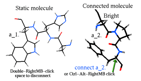
|
Option append will add selected molecule to the previously connected molecules
Note, that rotations/translations in the connect mode actually change the atomic coordinates of the selected molecules and keep the coordinate system unchanged in your graphics window.
To restore the usual global mode (i.e. all objects/molecules are disconnected and the mouse does not change their absolute positions, but rather the point of view), hit the Esc key when the cursor is in the graphics window. To restore the global mode temporarily press the Shift button.
Use: connect none to switch back to the global connection Examples:
read pdb "1eff"
copy a_1eff. # create something else in the scene
display ribbon a_*.
connect a_1eff.
# move it around now
connect none # disconnect
Connect to a Mysql database or database file |
connect molcart {S_host_user_pass_db|s_host s_user s_pass s_db} [name=s_connectionID]
Connects to the database server specified by the command parameters. It is possible to also specify the s_connectionID which will be assigned to the connection. Parameters returned by the Name(sql connect) may be used in this command.
connect molcart on
Reconnects to the current Molcart.
connect molcart refresh
Reconnects to Molcart using settings stored in user's preferences.
connect molcart filename=s_file [s_db] [name=s_connectionID]
Opens a Molsoft database file. Database name s_db and the s_connectionID may be specified.
connect molcart s_connectionID off
Disconnects specified Molcart connection. See molcart connection options for explanation
connect molcart local off
Closes all open database files.
See also: molcart, molcart connection options, list molcart, set molcart, Name molcart.
continue |
continue
skip commands until the nearest endfor or endwhile .
Example:
for i=1,5
  if i==3 continue  # do not print 3
  print i
endfor
See also: flow control statements.
convert |
[ Convert comp | Convert fragments | Convert mol | Convert and reroot ]
convert [os_nonICM] [auto|charge|exact|heavy|graphic|selection|simple|tether|selftether|tree=s_smiles] [s_objName]convert as_icmRootAtom [sstructure=as_scaffold] [auto] # root the icm-tree at as
convert rs_patches ..
the first convert command converts an incomplete non-ICM-object (e.g. object of type 'X-Ray'
resulting from the read pdb command) into a true ICM-object for which you may
calculate energy, build a molecular surface and perform all operations.
Options:
- auto - convert in place, preserve graphics and selections, e.g. convert auto selftether
- charge - transfer charge from the original
- exact - do not use the icm.res library by res name, convert as is.
- heavy - regularization (obsolete)
- graphic - transfer graphical attributes
- selection - transfer selection (as_graph)
- simple - special mode for disjoint chemicals
- tether - impose tethers to the original (use selftether for in-place or auto mode)
- tree= s_smiles - build the tree according to the smiles topology (small mol. convertion)
- selftether - imposes selftethers to the original coordinates, set field for the added heavy atoms ("_ADDED") and shifted upon conversion atoms ("_SHIFTED"), e.g. display cpk Select( a_// "_ADDED")
Description
There are two principally different modes of conversion.
In the default mode the program looks at the residue name and tries to
find a full-atom description of this residue in the icm.res file.
This search is suppressed with the exact option.
Hydrogen atoms will be added if the converted residues are known to the program and
described in the icm.res library.
If the object selection is omitted, the current object will be converted.
If default s_newObjectName is generated by adding number "1" to the source object name.
If s_newObjectName is the same as a name of the input object, the input object will be overwritten. (in-place conversion)
The default convert command is best used to convert PDB entries which have explicit residue descriptions and usually do not have hydrogen coordinates. In this mode each residue name is searched in the icm.res file and the coordinates of the present heavy atoms are used to calculate the internal geometrical variables (bond lengths, bond angles, phase and torsion angles) for the full atom model.
Every ICM atom will store the original coordinates as selftether (try show a_// and watch for the
ts= x , y , z record. Later these selftethers can be used with the "ts" term.
The exact option: converting protein with unusual amino-acids
Some pdb-entries may contain non-amino acid residues, or modified amino-acid
residues which do not need to be replaced by standard full atom library entries
with the same name . In this case use the exact option.
This option suppresses interpretation by short residue name and
converts the existing atoms and bonds in
single-residue molecules (amino acids in peptides and proteins will still
be extended by hydrogens upon conversion, to suppress that conversion
write the molecule as mol and read it back, then convert exact ).
Option exact may be necessary because chemical compounds with a
four-letter short name identical to one of the amino-acid residues, could be mistakenly
converted into an amino-acid with a corresponding name.
The charge option
Normally, upon conversion, the atomic charges are taken from the icm.res library entries.
Option charge tells the program to inherit atomic charges from the os_non-ICM-object.
For small molecules, use set charge, set bond type and, possibly,
build hydrogens before conversion of a new compound.
i_out will contain the number of heavy atoms missing from the pdb-template.
The graphic option preserves the graphical representations and colors as is.
The selection option preserves the atom selection bit during the conversion. Useful for in-place convert.
The sstructure= tree_substructure option makes sure that the tree is drawn through the substructure. It also needs a consistent entry atom provided as as_newRoot argument.
The auto option converts in-place preserving graphics and selection information. This is a convenient shortcut for the following combination:
- graphic
- selection
- s_newObjectName is set to the input object name
The smiles option ( an addition to auto option ) allows one to explicitly derive a tree structure from the smiles string. If the smiles string matches only part of the molecule then the rest of the tree will be built according to the default rules.
Additional cleanup
Actually more procedures need to be performed to prepare a functional object from crystallographic
coordinates, e.g. identifying optimal positions of added polar hydrogens, assigning the most
isomeric form of histidine , and finding a correct orientation of side-chain groups for glutamine
and asparagine.
We recommend the convertObject macro instead of the plain convert command to
achieve those goals.
Refining the model
To refine a model use the refineModel macro.
convertObject macro
The convertObject macro is a convenient next layer on the convert command.
The macro may convert only a few molecules out of your pdb file, optimize
hydrogens and do some other useful improvements of the model.
Output.
- the converted object
- i_out : the number of heavy atoms missing from the pdb-template,
- r_out : rmsd from the pdb-template atoms (non zero for residues with bad coordinates),
- i_2out : the number of deviating by more than 0.2A atoms heavy atoms,
- r_2out : the maximal deviation
- "built" -heavy atoms that were missing in a pdb (e.g. some lys and arg in 1qz5)
- "shifted" -atoms that shift after conversion (e.g. silly lysines in 1qz5)
Example:
read pdb "1crn"
display
as_graph = a_//c*
convert auto    # converts in-place preservinf slection and graphics
strip virtual
convert         # creates new a_1crn_1. object
If single atom is provided as an input selection it will be taken as a new ICM tree root. See convert and reroot for details.
See also:
- strip
- convertObject
- convert2Dto3D
- set cartesian
- selftether
- Select ( as s_tag )
Comparing convert, minimize tether and regularization. |
It is important to understand the difference between the convert command, the minimize tether command and the regularization procedure implemented in the macro regul .
All three create ICM-objects from PDB coordinates, but details of generated conformations and the amount of energy strain will differ.
We recommend to use convertObject macro for most serious applications involving energy optimization.
convert
- uses all-atom residue templates (including hydrogens) from the icm.res library
- creates temporary ICM-library descriptions for unknown residues
- makes geometry identical to the PDB coordinates: bond length and bond angles may be distorted.
- the converted structure will be energy strained because of common imperfections of the PDB entries and the hydrogen atoms added by the procedure
- C-alpha-only structures will not be properly converted because a special prediction algorithm is required to extrapolate the coordinates of all atoms from C-alpha atom positions.
- these objects are good enough for graphics, skin, secondary structure assignment, rigid body docking. They are not good for loop modeling and side-chain modeling.
- needs to be followed by polar hydrogen placement and histidine state prediction ( implemented in the convertObject macro )
minimize tether threading a regular polypeptide through an incomplete/gapped set of coordinates.
- you need to create a sequence file first and use the build command;
- you will need to create the missing residues manually, say, with the write library command;
- build will use all-atom residue templates including hydrogens, and will preserves the fixation;
- the linear chain with fixed idealized covalent geometry or, actually, any fixation you define, will be threaded onto the PDB coordinates in the best possible way;
- Ca-atom PDB structures will be handled properly if all backbone torsion angles are unfixed;
- the resulting ICM-object will be strained and will need further relaxation.
full regularization and refinement
- uses minimize tether to create the starting conformation;
- employs a multi-step energy minimization (annealing) of the structure to relief energy strain;
- these are the best objects that can create in ICM for further simulations.
Examples:
   read pdb "1a28.a/"           # reading just the first molecule
   convertObject yes yes no no  # the best way to prepare for docking
                                # convert + optimizes polar H, His and Pro

   read pdb "1crn"         # X-ray object, no hydrogens, no energy parameters
   convert                 # a_1crn_icm ICM-object will be created
   convert a_1. "new"      # a_new. ICM-object will be created
   convert a_1. exact      # keep modified residues as is

   read mol2 s_icmhome+"ex_mol2"
   set object a_catjuc.
   build hydrogen
   set type mmff
   set charge mmff
   convert
Creating a multi-part molecule in which parts are separately controlled. |
If you want to create a local "epitope" of a protein with chain fragments around a particular area, it can be done with the
convert rs_fragments
command. This command will create a molecule divided into fragments and each fragment will start from virtual atoms vt1 and vt2 and will be controlled with 6 virtual variables. The first vt1 of the second, third etc. fragments will be connected to the first real atom of the first fragment. Example:
read pdb "1crn"
convert a_/4:10,12,27:33,41:45
Nof( a_m//vt1 ) # the number of pieces
show v_/P1/V  # the pos. variables of the 1st part
show v_/P2/V  # the pos. variables of the 2st part
display ribbon
color ribbon a_/P3  # showing the 3rd part
This operation is useful to create a local patch object for docking of global optimization.
Converting a chemical compound from a mol/sdf or mol2 files. |
To convert a chemical from GUI menus, follow these steps:
- make sure that bond types and formal charges are correct
- select the MolMechanics.ICM-Convert.Chemical menu item, check the parameters and press OK. Normally to convert from 2D to 3D you need to optimize the ligand. ICM will perform a multiple start global optimization using the MMFF94 force field ( internally it runs the convert2Dto3D macro ). If you want to preserve the geometry, select the keepGeometry option.
Command line conversion To perform the same conversion in a batch run the convert2Dto3D macro, or, to make a conversion without full optimization from a command line or script, issue the following commands:
# assuming that bond types and formal charges are correct
build hydrogen
set type mmff
set charge mmff
randomize a_//!vt* 0.01 # sometimes it helps to avoid singularities
convert
set v_//T3 180.  # making flat peptide bonds
fix v_//T3       # optional
Example of geometry optimization:
read mol input = String( Chemical("C(C(O)=O)N1C(C(=Cc2ccc(c3ccccc3[Cl])o2)SC1=S)=O"))
convert2Dto3D a_ yes yes yes yes
list convert2Dto3D
Converting a chemical compound and rerooting the tree at the same time |
convert as_rootAtom [auto]
if an atom selection is provided instead of the object selection, the tree will be rerooted to the selected atom. The converted molecule will have the as_rootAtom located at the root of molecular tree so that it is convenient to modify another molecule with the converted molecule.
auto option behaves as in normal convert command. It preserves selection and graphics and preforms in-place conversion.
If you need to reroot an ICM object, do the following:
- strip it to a non-ICM object: e.g. strip virtual
- re-root and convert, e.g. convert a_//hb1 .
Example:
build smiles "C(=CC=C(C1)C(=O)O)C=1"
display wire
wireStyle = "tree"
strip a_ virtual
convert a_//h31 auto   # converts from a new root
copy |
[ copy-object ]
copies stuff which CANNOT be copied by direct assignment such as: a=bcopy os [ s_newObjectName ] [delete|display|graphic|selection|stack|strip|tether]
creates a copy of os_ with the specified name. Default source object is the current object.
The default name is "copy" (object a_copy. )
Options:
- delete forces the command to overwrite the object with the same name if there is a name conflict.
- display or graphic copy the display attributes of the parent
- selection copies named selections defined on the parent object into the copy
- stack copies internal stack of the object (see store-object-stack) (the stored stack is not copied by default)
- strip applies the strip operation to the copied object. The stripped object has a PDB type and is much smaller in memory.
- tether applies tethers from the source object to the atoms of the copy-object. For further refinement see the refineModel macro.
Examples:
 read pdb "1crn"
 copy a_           # creates a_copy.
 copy a_1. "aaa"   # creates a_aaa.
 read object s_icmhome+"crn" # read ICM object
 copy a_ strip delete tether # create a_copy. and tether to it
crypt |
crypt key= s_password { s_fileName | string= s_string }
encrypts the file s_fileName or string s_string in place (the size of the encrypted file/string is exactly the same), adds extension .e to the file name. If string is encrypted, its name is not changed. Apply the operation again to restore the file or string. You may encrypt both text and binary files. Note that this command has nothing to do with the unix crypt utility. ICM uses different algorithm.
Examples:
crypt key="HeyMan" "_secretScript"    # encrypt and create *.e file
crypt key="HeyMan" "_secretScript.e"  # decrypt it
ss="Secret rumour: Div(Rot(F))=0 !"
crypt key="fomka" string = ss  # encrypt
show ss
crypt key="fomka" string = ss  # decrypt
show ss
Date data-type |
A basic ICM class for arrays of date objects
See also: Date.
delete ICM shell objects |
[ Delete shell object | delete alias | Delete molcart | Delete plot | Delete selection | Delete variable | delete atom | delete directory | delete file | Delete session | delete hydrogen | delete object | delete molecule | delete bond | delete boundary | Delete column table | delete conf | delete drestraint | delete label | Delete label chemical | delete link | delete map | delete sequence | delete site | delete sstructure | Delete site alignment | delete disulfide bond | delete peptide bond | delete stack | Delete stack object | Delete element | delete table | delete term | delete selftether | delete tether | Delete parray | Delete chemical selection ]
delete shell objects or their parts.delete ICM-shell object |
delete [ alias ] [ alignment ] [ factor ] [ grob ] [ iarray ] [ integer ] [ logical ] [ macro ] [ map ] [ matrix ] [ profile ] [ rarray ] [ sarray ] [ sequence ] [ string ] { name1 | s_namePattern1 } name2 ...
delete all # to delete all shell objects not marked with a no delete flag
ICM-shell objects have unique names; to delete some of them just type
delete [ mute ] { icm-shell-objectName1 | s_namePattern1 } icm-shell-objectName2 ...
You may use name patterns with wildcards (see
pattern matching)
and add explicit specification of the ICM-shell object type,
if you want the search to match only the objects of particular type.
If the ICM-shell object type is not specified, all the shell-variables
will be considered.
Option mute will temporarily switch off the l_confirm flag.
delete class
delete string className
delete string command | html
to delete icm-command files or html-documents loaded into ICM
delete rarray view
to delete all the views (returned by the View() function)
Examples:
   delete aaa           # delete ICM-shell object aaa
   delete a b c         # delete ICM-shell objects a, b and c
   delete "*"           # delete ALL ICM-shell objects added by user
   delete "mc?a*" mute  # delete ICM-shell objects matching the pattern
   delete rarrays       # delete ALL real array
   delete objects       # delete ALL molecular objects, same as delete a_*.
   delete rarray "a*"   # delete real arrays starting with 'a'
Deleting array elements To delete a selection of array elements specified as an index expression or an integer array of indexes, use the expression from the following example:
  a={1 2 3 4 5 6}   # we want to delete elements from it
  a=a[2:4]          # retain only elements 2:4
  a={1 2 3 4 5 6}
  a=a[{2,3}//{5,6}] # retain only 4 elements elements
  a=Count(100)
  a=a[Count(1,10)//Count(21,30)]  # retain ranges 1:10 and 21 to 30
Deleting table elements table rows can be deleted directly with the delete command, e.g.
 delete t.A>1
 delete t[{1 3 5}]
delete alias |
delete alias
see alias delete alias_name . Example:
alias ls list
alias delete ls
Delete from database |
delete molcart table s_dbtable [connection_options]
Deletes table from Molcart database with all index tables, related indexes and metadata.
Database connection may be specified by connection_options
Delete plots from the table |
delete plot table [name=s_handle]
This command deletes from the table all plots or only the plots with the specified name (see make plot).
ICM table plots are stored in the table header as an sarray T.plot, so 'delete plot T' is identical to 'delete T.plot'
delete selection variable |
delete as_selectionName
or
delete vs_selectionName
delete named variable with atom or v_ selections. The number of named selections is limited to about 10 in each category, therefore you may need to delete them from time to time.
Important: keep in mind that deleting the named selection is not the same as deleting actual objects, molecules or atoms selected by them. To delete atoms selected by a named variable in an non-ICM object, add keyword atom (see delete atom nameSelection )
Examples:
 build string "ASFGD"      # build a molecule
 vsel = v_//phi,psi    # this is a vselection
 delete vsel

 asel = a_//c*,n*      # this an aselection (atom selection)
 delete asel           # delete variable asel, do not touch the atoms
 delete atom asel      # delete atoms in a non-ICM object
Delete array elements |
delete variable array {i_elementNumber|I_elementNumbers}
delete one or more elements from any array. If the array is a column in a table T, use the delete T[i] command which can delete both a single row, e.g. delete t[2], or a row selection.
Examples:
a={1 2 3}
b={1. 2. 3.}
c={"a" "b" "c"}
delete variable a 2  # deletes the 2nd element of the array
show a
 {1 3}
delete variable b 2
delete variable c 2
#
a = Count(100)
delete variable a Count(50)*2 # deletes even numbers
delete variable pairdistArray I_pos
Removes elements at positions I_pos from the array
delete atom |
delete as_atoms
delete atoms as_namedSelection
delete selected atoms in a non-ICM object. The selection
here must be a constant atom selection, rather than a
named selection (e.g. you can say delete a_/1:10/*
but NOT aaa = a_/1:10/* , delete aaa ).
To delete a named variable, use delete atom name
Example:
  read pdb "1crn"
  delete a_/1:10/*

  aaa = a_/18:20
  delete atom aaa
See also: build atom , delete hydrogen
delete directory |
delete directory s_Directory
delete directory. Example:
delete directory "/home/doe/temp/"See also:
| command | comment | unix equivalent |
|---|---|---|
| delete system s_f1 | delete a single file | rm file1 |
| copy-systems_f1 s_f2 | copy a single file | cp file1 file2 |
| rename system s_f1 s_newname | rename/move a single file | mv file1 file2 |
| set directory s_dirname | change directory (cd) | cd dirname |
| make directory s_dirname | make a directory | mkdir |
| Path ( directory ) | returns the path to the current directory | pwd |
| Sarray ( s_filename_filter directory [ all ] ) | returns the file list array, all goes to subdirectories | ls -1 [-R] namepattern |
delete file |
delete system s_fileName s_fileName ...
delete external file.
Example:
delete system "/tmp/aaa"
See also other internal icm equivalents of the system commands that allow to avoid new threads.
| command | comment | unix equivalent |
|---|---|---|
| copy-systems_f1 s_f2 | copy a single file | cp file1 file2 |
| rename system s_f1 s_newname | rename/move a single file | mv file1 file2 |
| make directory s_dirname | make a directory | mkdir |
| set directory s_dirname | change directory (cd) | cd dirname |
| delete directory s_dirname | delete an empty a directory | rmdir |
| Path ( directory ) | returns the path to the current directory | pwd |
| Sarray ( s_filename_filter directory [ all ] ) | returns the file list array, all goes to subdirectories | ls -1 [-R] namepattern |
delete history lines |
delete session
deletes all previous history lines. Example:
call _macro
delete session
delete hydrogen |
delete hydrogen as
delete hydrogen chem [all]
delete selected hydrogen atoms in a non-ICM object or a chemical array. See also
build hydrogen. To delete hydrogens
in an ICM object, strip it first.
When the hydrogens are deleted in a chemical array, the default is to preserve the chiral hydrogens in fused rings (the regular chiral hydrogens will still be deleted). To delete all hydrogens use option all . In the latter case when the hydrogen carrying the stereo bond is deleted for all heavy atoms including fused rings and the stereo bond will be reassigned to one of the heavy atom neighbors.
Example:
build string "ASD"
strip # makes a non-ICM object
delete hydrogen a_/2,3/h*
#
group table t Chemical("[C@@](C)(N)[H])O") "mol"
delete hydrogen t.mol all # all hydrogens gone
delete object |
delete { object | os }
delete molecular object. Make sure that you specify an object selection ( a_1crn. is correct, a_1crn.* or a_1crn.//* is INCORRECT.) To delete an object from a selection variable ( as_out,as2_out or as_graph, or any use defined aselection variable), use delete atom as_namedSelection (e.g. delete atom as_graph ) or specify the selection level explicitly.
Examples:
   delete object          # delete ALL molecular objects
   delete a_*.            # delete ALL molecular objects
   delete a_2,4.          # delete objects number 2 and 4
   delete a_2a*.          # delete objects with names starting from 2a

   read pdb "1crn"        # load crambin
   convert                # create the second object named 1crn_icm
                          # from the pdb object
   delete a_1.            # delete the 1st pdb-object
   delete Object( as_graph )  # graphical selection
delete molecule |
delete [ molecule ] ms
delete separate molecules from molecular objects. The integer reference number(s) of molecule(s) which can be shown by the show molecule command and used in molecule selections are redefined after deleting or moving molecules from or in the ICM-tree, respectively.
To delete a molecule from a selection variable (as_out,as2_out or as_graph, or any use defined aselection variable), use delete atoms as_namedSelection (e.g. delete atom as_graph ) for non-ICM objects, or use the Mol function to specify the selection level explicitly (e.g. Mol( as_graph ) ).
Examples:
   read pdb "2ins"        # load insulin with water molecules
   delete a_2ins.w*       # delete water molecules
   delete atoms as_graph  # deletes selected non-ICM atoms/molecules
   delete Mol( as_graph )  # deletes selected non-ICM atoms/molecules
delete bond |
delete bond as_singleAtom1 as_singleAtom2
delete a covalent bond between two selected atoms. This command is used to correct erroneous connectivity guessed by the read pdb command. It is particularly important when you are going to create a new ICM-residue using the write library command and the entry to it in the icm.res or your own residue file (it has the same format). In interactive graphics mode you may type delete bond and then click two atoms with the CTRL button pressed.
Examples:
   read pdb "newmol"              # automatic bond determination is not perfect
   delete bond a_/3/cg1 a_/5/ce2  # disconnect two carbon atoms
See also: make bond and make bond atom_chain .
delete boundary |
delete boundary
an auxiliary command to free additional memory allocated by the make boundary command.
delete columns in a table |
delete column T [inverse] [ I_cols | S_cols | selection | iarray | rarray | sarray | parray | i_from [ito] ]
delete columns in a table T. Option inverse keeps the specified columns and delete the rest. You can select columns in multiple ways:
- by array of indexes : e.g. 3//4//5
- by array of column names :
- by GUI selection:
- by column type: e.g. rarray sarray
- by column index range: e.g. 3 (meaning all except column 1 and 2)
Example:
   add column t 1//1 2//2 3//3 'a'//'b' 5.5//5.5 6.6//6.6 's'//'s'
   delete column t 3  # starting from column 3
   delete column t 3 5 inverse  # all except 3,4,5
   delete column t iarray rarray
   delete column t 't.A'//'t.B' inverse # delete all except columns 'A' and 'B'
See also: rename column tab ..
delete conf |
delete conf i_stackConfNumber [os_obj]
delete conf i_confNumberFrom i_confNumberTo [os_obj]
delete conf I_stackConfNumbers [os_obj]
delete a specified conformation from the stack or a series of conformations
starting from i_stackConfNumber to i_stackConfNumberTo .
An integer array of indices can also be provided.
if the os_obj argument is provided the changes above will be applied to the local stack in the object.
See also:
delete drestraint |
delete drestraint [ as_1 [ as_2 ] ]
delete distance restraints formed between specified atom selections as_1 and as_2. If no selection is specified all distance restraints are deleted
Examples:
delete drestraint a_mol1 a_mol2 # intermolecular restraints
delete label |
delete label [ i_StringLabelNumber ]
delete graphics string label (text in the graphics window). These strings have no unique identification names, they are just numbered. Numbers are compressed as you delete some labels from the middle of the list.
Examples:
   delete label # deletes all labels
   delete label 1  # delete the first displayed label
See also:
| show label | to find out the label number and |
| display label | to create and display a string label. |
delete labels from 2D chemical spreadsheets |
delete label chemarray [all] [index=I_]
deletes atom annotation in 2D chemical spreadsheet. Without the all option the command will only remove labels from the selected atoms, otherwise all labels will be removed. The selection can be done in the GUI and it appears as a green halo around select atoms.
Example:
# create annotated chem table
add column t Chemical({"CCCCN","CCCNCCC","CC(=O)O","C(=O)O"})
add column t Predict( t.mol "MolpKaBase" ) name="pkab"
add column t Predict( t.mol "MolpKaAcid" ) name="pkaa"
set label t.mol t.pkab window = {0.,14.}
set label t.mol t.pkaa window = {0.,14.}
# now delete it
delete label t.mol all
See also: set label chemical
delete link |
delete link ms
delete links to sequences and alignments for selected molecules
delete link variable
delete all groups of linked variables (e.g. unlink the variables), see also link variables .
delete map |
*delete { *map | s_mapName } delete s_mapName or all maps.
delete sequence |
delete sequence [ seq_1 seq_2 .. ]
delete sequence { selection | compress | protein | peptide | nucleotide | unknown | swiss }
delete sequence i_minLen i_maxLen
(to delete a sequence form alignment use the only option, see below).
- selection : delete the sequences selected through GUI.
- compress : delete the sequences not included in the alignments, i.e. freely floating sequence not included in any alignments, (compare with the compress option of delete )
- protein or peptide will delete only amino-acid sequences,
- nucleotide will delete only DNA or RNA sequences,
- unknown : delete sequences with more than 20% of 'X' or 'x' residues. Note that this option changed its meaning. Previously it was same as compress.
- by sequence length, (e.g. delete sequence 1 50 )
delete sequence n_seq_at_the_end_of_seq_list
delete sequence [ i_minLength i_maxLength ] # delete OUTSIDE range.
- no arguments: delete all ICM-sequences
- one integer argument: delete last n sequences from the sequence list
- two integer argument: delete sequences shorter than i_minLength or longer i_maxLength
Deleting some sequences from an alignment but not deleting sequences themselves
delete alignment only selection
delete alignment only seq1 seq2 ...
To delete sequences selected via the graphics user interface from an alignment without deleting them from the shell. Example
  delete sh3 only Fyn
  delete sh3 only selection
delete site |
delete site seq [{s_Site|i_number|I_numbers|pattern=s}]
delete site ms1 [{s_Site|i_number|I_numbers|pattern=s}]
delete site rs
delete the sites of the selected molecules. The sites can be specified
by their name, or number, or residue selection. All sites are deleted by default.
Example:
   nice "1as6"          # has 3 sites, one in each molecule.
   delete site a_1.1 {1}
   delete sites         # delete all of them
See also: site
delete sstructure |
delete sstructure seq_1 seq_2 .. delete sstructure select
delete the assigned secondary structure to prepare the sequence for the secondary structure prediction (see the Sstructure function).
The selection option allows one to delete secondary structure only for the sequences selected through GUI.
delete site in alignment |
delete site ali [i_number] [I_box]
deletes annotation in the alignment by i_number or inside the I_box.
See also: set site alignment
delete disulfide bond |
delete disulfide bond [ all ] [ { rs_Cys1 rs_Cys2 | as_atomSg1 as_atomSg2 }]
delete specified or all disulfide bridges in ICM objects.
Examples:
           # SS-bond specified by residue, or
   delete disulfide bond a_/15 a_/29
           # by atoms
   delete disulfide bond a_/15/sg a_/29/sg
           # remove all SS-bonds in the current object
   delete disulfide bond all
See also:
make disulfide bond and (important!)
disulfide bond.
delete peptide bond |
delete peptide bond [ as_N as_C ]
delete specified extra peptide bonds in ICM objects (e.g. imposed to form a cyclic peptide).
Example:
delete peptide bond a_/15/c a_/29/nSee also: make peptide bond and peptide bond.
delete stack |
delete stack
delete the main stack of conformations in ICM shell. Be careful, there is a single share stack in the shell (deleted by this command) and each ICM object can also store a compressed stack of conformers.
See also read stack, read stack, write stack, and delete conf.
delete conformational stack inside an object |
delete stack os
deletes the compressed stack inside the specified object.
See also:
- store stack object
- load stack object
- montecarlo .. store
- set object .. stack
- Exist ( os1 stack )
delete parray elements |
delete parray[i_index]
delete parray[I_index_list]
deletes specified elements from a parray.
Example:
C = Chemical({"C","CC","CCC","CCCC","CCCCC"})
delete C[{1,3,5}]
delete C[1]
delete table |
delete { T_table | table_expression }
delete the specified complete table or just the entries selected by the expression.
Examples:
   group table t {1 2 3} "a" {4. 5. 7.} "b"
   delete t.a == 2       # the second entry
   show t
   delete t[2]           # the second entry
   show t
   delete t              # the whole thing
   group table t {1 2 3} "a" {4. 5. 7.} "b"
   delete t.a > 1          # 2nd and 3rd
delete term |
delete term s_terms
switch off the specified terms of the energy/penalty function.
Examples:
delete terms "tz,sf" # do not consider tethers and solvation contributions
delete selftether |
delete selftether [ as]
deletes internal tethers for selected (or all atoms)
See also:
delete tether |
delete tether [ as]
delete tethers of the specified atoms ( as_ ), if no selection is specified all tethers in the current object are deleted.
delete tether loop [ as] - this tool deletes tethers for residues flanking insertions and deletions (one residue on each side), as well as N- and C- termini. The tool is used to help the minimize tether command to build a more relaxed loop or end.
delete a tree from a table header array |
delete variable treeParray i_treeIndex
deletes a tree object (generically considered as a parray )
Example:
make tree T
delete variable T.cluster 1
delete selected chemical fragments |
delete chemical chemarray
deletes selected parts of the chemicals. See select chemical command.
display |
[ display model | Display new | Display offscreen | display origin | Display rotate | display stack | display box | display clash | display drestraint | display gradient | display grob | Display grob label | display hbond | Hbond color | display label | display map | Display trajectory | display ribbon | display site | Display skin | display slide | display string | display tethers | display volume | display window | Display gui ]
display molecules or graphical objectsdisplay model |
display [wire|cpk|ball|stick|xstick|surface|skin|ribbon [base]] [as [as_2]] [ color ] [virtual] [center [center_options]]
display [transparent] [stick|skin|ribbon [base]] [as [as_2]]
display specified graphics primitives for selected atoms or residues.
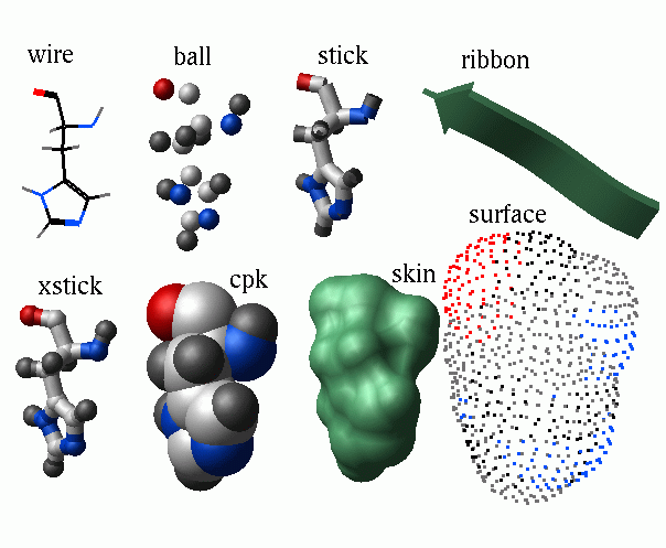
|
Once something is displayed and your cursor is in the graphics window you may rotate, translate, zoom and move both clipping planes with the mouse and keystrokes.
To refer to the base part of DNA/RNA represented as ribbon , use the additional specifier called base, which can be separately displayed and colored. E.g.
 makeDnaRna "ACTG" "mydna" yes yes "dna"
 display ribbon
 color ribbon base a_1 blue
Display surface atoms may be defined by TWO arbitrary selections (it would mean: display surface of atoms as_1 as they are surrounded by atoms as_2 ) Note that the GRAPHICS.hydrogenDisplay preference may affect the displayed atoms. To be able to display all atoms set GRAPHICS.hydrogenDisplay to "all".
Defaults: wire representation, all atoms (corrected by the GRAPHICS.hydrogenDisplay), coloring according to atom type.
color options
The color can be specified by a number of ways (see the color command for a more detailed description) : Color (e.g. red ), s_Color (e.g. "red"), numerical color:
i_Color | r_Color | I_Color | R_Color [ window= R_2minmax ]
The window array of min and max values allows one to clamp the value you want to map to a color to the specified range.
Other options:
center : will perform the center command on the displayed object(s).
transparent : will display the ribbons, skins or sticks as transparent objects,
read pdb "1crn"
display transparent ribbon
display skin transparent
display surface refresh : will rebuild the surfaces with new GRAPHICS.surfaceDotSize values.
intensity= r_fraction : renders the image with fractional intensity by merging the source display image with the background.
virtual : additionally displays the coordinate axes, virtual atoms and virtual bonds starting from the origin. It is a good way to visualize the whole ICM molecular tree as it grows from the origin. This option is applicable only to the ICM molecular objects.
More examples:
 build string "AFSGDH;QWRTEY"       # two peptides
 display                        # display current object and color atoms
                                # according to atom type
 display a_1 red                # display the first molecule and color it red
 display skin a_/5 a_* yellow   # display skin of the 5th residue
                                # as surrounded by all the atoms
 display ribbon                 # display ribbon for all the residues

 read pdb "2drp"                # a pdb file
 assign sstructure a_a/123:134,153:165 "H"       # No sstructure in 2drp
 assign sstructure a_a/109:114,117:121,141:144,147:151 "E"
 display a_a ribbon red                          # two Zn-fingers
 display a_a/113,116,143,146/!n,c,o xstick blue  # Cys residues
 display a_a/129,134,159,164/!n,c,o xstick navy  # His residues
 display a_m,m2 cpk magenta                       # Zn-atoms
 adna1=a_b//p,c3['],c4['],c5['],o3['],o5[']      # two DNA chains
 adna2=a_c//p,c3['],c4['],c5['],o3['],o5[']
 display adna1 xstick white
 display adna2 xstick aquamarine
 display adna1 adna1 surface white
 display adna2 adna2 surface aquamarine
 center
 display "Zn-finger peptides complexed with DNA" pink

# display 4 chains of insulin as 4 thick worms colored from N-to C-terminus
 read pdb "2ins"
 color background blue
 assign sstructure a_/* "_"  # thick worm representation
 GRAPHICS.wormRadius= 0.9
 display a_/* ribbon only
 color a_1/* Count(1 Nof(a_1/* )) ribbon
 color a_2/* Count(1 Nof(a_2/* )) ribbon
 color a_3/* Count(1 Nof(a_3/* )) ribbon
 color a_4/* Count(1 Nof(a_4/* )) ribbon

# examples of DNA and RNA ribbons
 nice "4tna"
 resLabelStyle = "A"
 display residue label
 color residue label a_/?u gold # ??u also selects modified Us
 color residue label a_/?a red
display new: refresh or unclip view |
display new
display restore
display restore plane
commands to mimic some of the interactive controls.
These commands are primarily used in GUI commands ( see icm.gui file) and scripts/macros.
new :
rebuilds some graphical representations (e.g. your as_graph has been
changed in the shell and you need to refresh the image, or
you changed the orientation and want to redisplay the labels
elevated above the skin surface by resLabelShift ).
restore :
a softer action than new .
restore plane :
moves the clipping planes beyond the displayed objects
(keystroke: Ctrl-U, or the 'Unclip' button) .
display off-screen |
display off [ i_Width i_Height ]
Sometimes you want to generate some images in a script without opening an explicit graphics window. The display off command opens an off-screen rendering buffer of i_Width by i_Height size in pixels, in which all the usual display/color/undisplay/center commands work as usual. NOTE: one cannot have both off-screen and on-screen displays in one ICM session.
An example script (can also be performed interactively):
   display off 400 300
   nice "1est"
   rotate view Rot( {0. 1. 1.} 50.)
   write image "est1"
   unix xv est1.tif
   set window 700 800  # NB: 'center all' will be applied
   write image "est2"
   unix xv est2.tif
   display a_/4/o cpk
   center a_/3,4
   write image "est3" rgb
   unix xv est3.rgb
   build string "se ala trp"
   display off 400 300
   display skin
   write image "est3" rgb delete
   unix xv est3.rgb
display origin |
display the axis of the coordinate frame. The length of the arrows is defined by the axisLength parameter. Use undisplay origin to undisplay it. E.g.
 read pdb "1crn"
 display
 display origin
 undisplay origin
Setting rotation or rocking mode |
display rotate [on|off] [ i_NofCycles ] [pause]
The graphics view can be set so that molecule is continuously rotating or rocking, but the ICM session remains interactive. This mode can be set with the above command. The style of continuous interruptable movement is controlled with the GRAPHICS.rocking preference. Specifying the number of rotation or rocking cycles i_NofCycles is useful for movie making. The pause option forces the command to finish the requested number of rotations before proceeding to the next commands, as opposed to just launching the rotation and proceeding with the rest of the script.
Example:
GRAPHICS.rocking = "xY-rocking"
display rotate on 3 # three cycles
See also:
write movie , GRAPHICS.rocking
display stack |
display stack [ os_withStoredStack ] [iFrom iTo] [loop [=nCycles]] [r_NofInterpolationFrames [simple|cartesian]] [center] [reverse] [sstructure] [auto]
interpolated display of conformational stack of its parts. Aruments and options:
- optional os_withStoredStack . If this argument is missing, the global stack will be used. With the argument the built-in local object stack will be played out.
- optional start and end frames: iFrom iTo
- option loop [ = nCycles ] : the command makes a video loop and repeats it 99999 times. Optional nCycles redefines the number of repetitions.
- r_NofInterpolationFrames [ simple | cartesian ] ] (e.g. 10.0 cartesian ) : determines the number of intermediate frames.
The following interpolations are currently provided:
- simple : just wait for the specified number of frames
- cartesian : perform linear interpolation between stack conformations
- option center : centers on the displayed atoms
- option sstructure : recomputes secondary structure for each stack conformation.
- option auto : extracts the number of cycles (1 or endless loop) and the number of interpolated frames ( no interpolation or a fixed number of interpolated frames) from the stack itself. The two parameters can be set with the set stack os loop|fast [off] command. The GUI interface for the object stack display uses the auto option.
- option reverse : toggles iteration between first and last frame back and forth. (Doesn't jump from the last frame to first, instead goes reverse to the first)
Example:
  build string "ASDFW"
  montecarlo v_//x* mncalls=10 vwMethod=2 # create a conformational stack
  display xstick cpk  only
# the previous commands just prepare stack and display
  display stack 20. cartesian loop=4 center # repeat 4 times and stop
Another example in which the displayed trajectory is dumped into a movie file.
# make the same preparations
  write movie "peptamovie" on exact
  display stack 20. cartesian loop=1 center # repeat 4 times and stop
  write movie exit
The display stack command is somewhat similar to the display trajectory command. The display stack command has the following benefits:
- it recomputes the skin if the skin is present
- does not mess up the C-terminus in case of local deformations
- does not save or use any external files.
- it allows easy looping with the loop [= nCycles ] option.
See also:
display box |
display box [ R_6boxCorners ]
display graphics box specified by x,y,z coordinates of two opposite corners of a parallelepiped. This box can be resized and translated interactively with the Left and Middle mouse buttons:
- Resizing: Grab a corner of the box with the Left-Mouse-Button and drag it to resize the box
- Translating: Grab a corner or a center of the box with the Middle-Mouse-Button and translate
See also the
Box () function which returns six parameters describing the box.
Examples:
   build string "se ala his gly met" # a peptide
   display
   display box                      # the default box
   display box {0. 0. 0. 2. 2. 2.}  # define position/size
   display box Box(a_/2 )           # surround the a_/2 by a box
   display box Box(a_/2 1.2)        # or add 1.2A margin
display clash |
display clash [ as_1 ] [ r_clashThreshold ]
display all the interatomic distances for selected atoms which are shorter than the sum of van der Waals radii multiplied by the r_clashThreshold parameter. The default value is taken from the clashThreshold variable. Initially it is set to 0.82 but can be redefined. IMPORTANT: this will work only for the ICM-objects. For hydrogen bonded atoms the threshold is additionally multiplied by 0.8. Use the show energy "vw" command (and pay attention to the current fixation) to precalculate interaction lists.
This command may show some irrelevant short contacts. calcEnergyStrain , display gradient , etc. seem to be more informative.
See also: GRAPHICS.clashWidth , clashThreshold , show clash, undisplay and atom energy gradient (force) analysis with: show a_//G or display a_//G.
Example:
 read object s_icmhome+"crn"
 show energy "vw"
 display a_
 display clash                  # all clashes, default clashThreshold=0.82
 undisplay clash
 display clash a_/11 0.95  	# distances < (R1+R2)*0.95
# this is an alternative method which analyzes the gradient
 selectMinGrad = 100.   	# analyzes forces greater than 100
 display ribbon grey
 display Res( a_//G )
 display gradient a_//G
 color Res( a_//G ) ribbon magenta
display drestraint |
display drestraint as
displays drestraints, disulfide bonds, and peptide bonds imposed on selected atoms.
See also: read drestraint, set drestraint, make disulfide bond, make peptide bond, make drestraint.
Example:
  build string "se ala his trp ala gly gly"
  display
  set drestraint a_/1/hn a_def.a1/6/o 2
  show energy "cn"
  display drestraint
  minimize "vw,14,to,cn"
display gradient |
display gradient as
display vectors of energy derivative with respect to atom positions or selected atoms as_ .
Important: the gradient must be pre-calculated by using one of the following commands: show energy or minimize . The values of gradient components (lengths of vectors for each atom) can be shown by show gradient as_. When a gradient vector is displayed, two transformations are performed: it is scaled and colored to represent the range of values in the most convenient and natural way while still being able to deal with a wide range of gradient values from negligible to 10 to the thirtieth power, as may be the case for a strong van der Waals clash. When all gradient vectors are under 20 kcal/mole*A they will be colored by the "cold" colors (blue...green...yellow) and will be assigned a length less than 2 Angstroms. If you see a red and long vector you may have a problem. Check it by zooming in and using show gradient as_. You can also select only atoms with gradient greater than the threshold value selectMinGrad by typing a_//G and display only specified strained atoms. It helps to get rid of little blue arrows for unstrained atoms.
Examples:
 build string "ala his trp glu leu"
 randomize v_//phi,psi
 show energy
 selectMinGrad= 20.
 display a_
 display gradient a_//G
display grob |
display grob [ solid ][ smooth ][ dot ][ reverse ] [ transparent ]
display g_Name1 g_Name2 ... options
display grob selection ... options
display all, specified, or graphically selected graphics object(s) . They are referred to as grob in the ICM-shell and as "3D meshes" in the GUI interface. The display grobs command will display all existing graphics objects. Options:
- dot will show only dot-vertices of the object.
- reverse to invert lighting; this option will change directions of the grob surface normals (will turn the grob inside-out)
- smooth enforces the Gouraud shading method to smooth the solid surface.
- solid allows solid surface representation of the object and requires that the original object has information about triangles forming the solid surface.
- transparent makes solid grob transparent
Examples:
   read matrix s_icmhome+"def.mat"    	# 2D sin(r^2)/r^2 function of a grid
   make grob solid def      		# convert matrix into a graphics object g_def
   display g_def smooth     		# a hat of the 22st century
   rotate view Rot({1. 0. 0.}, 45.)     #
   display g_def reverse    		# shine light from inside the head
   display grob smooth transparent 	# like Lenin in Mausoleum
set font of a 3D label |
display g_label [bold ] [ italic ] [ underline ] i_Size [font=s_FontName] [rgb=R_3rgb|"#xxyyzz"]
displays g_label text (technically it is a grob with a single point and associated text) in a particular font.
Example:
read pdb "1crn"
display a_
label3d = Grob("label",Mean(Xyz(a_/3,4)), "3D label for res 3,4")
set font label3d times 36 rgb="#00ffdd"
display label3d
select edit label3d # makes it movable, press Esc to get rid of the cursor
display hbond |
display hbond [ as ] [ r_maxHbondDistance ] [ only ]
Only hydrogen bonds of the current object may be displayed. Before calling this command, you should use any of the following commands: show hbond, show energy, minimize to calculate the list of hydrogen bonds. The real argument r_maxHbondDistance defines an upper bound of the distance between a hydrogen and a potential hydrogen acceptor to place the pair to the hydrogen bond list. (Default value of r_maxHbondDistance parameter is 2.5 A.) The list is recalculated for each new loaded molecular object. Hydrogen bonds on display are colored according to their hydrogen-acceptor distances. The option only allows one to display hydrogen bonds without corresponding molecular object. Longer and shorter H-X distances in the hydrogen bond are color-coded, from red to blue, respectively.
For ICM object the hydrogen bonds are calculated much faster because the atom pairs are precalculated. However, the displayed hydrogen bonds will then depend on how the model was fixed. No hydrogen bonds will be shown inside rigid bodies.
The color or hydrogen bonds will be calculated according to a calculation involving the effective lone pair density (see hbond color ).
See also: undisplay hbonds, show hbonds.
Strength and color of a hydrogen bond |
The hydrogen bonds created or displayed with the make hbond or display hbond commands are colored according to the estimated 'strength' of this hydrogen bond. This is just an estimate since the energy of hydrogen bond is not easily decoupled from the van der Waals and electrostatic contributions between the hbonded atoms and their immediate environment. In ICM the strength is estimated using the following procedure described in J Med Chem. 2003 Jul 3;46(14):3045-59.
For a hydrogen bond acceptor atom A(i) and a hydrogen atom H(j) located at rj, the hydrogen bonding interaction was estimated
Fang(phi)Fdist (rLPi -rj)
, where phi is an angle formed by the hydrogen bond acceptor atom, hydrogen, and the hydrogen bond donor, and rLPi is the radius vector of the center of the lone electron pair (LP) closest to the hydrogen. The angular function used was defined as Fang = 1 - cos(k*phi) . Parameter k is accessible as GRAPHICS.hbondAngleSharpness in the shell. Distance function Fdist (rLPi-rj) was constant (1.0) within LHB/2 from the lone pair center and dropped as
exp( -(((rLPi - rj)/LHB) - 0.5)2 ) .
beyond that distance, where LHB is the characteristic range of hydrogen bonding interaction (value of L=1.6 �was used). Lone pair centers were placed at 1 �from the hydrogen bond acceptor atom, assuming symmetrical planar trigonal configuration for sp2 atoms and tetrahedral configuration for sp3 atoms. The resulting functional dependence reflects (at least qualitatively) the physical nature and observed statistics of the hydrogen bond interactions. The interaction is maximized when the hydrogen atom is pointing directly to the acceptor atom along a lone pair axis and drops quickly as the hydrogen is moved farther away. The strength declines more gradually as the hydrogen moves out of the LP axis or, as hydrogen bond donor, hydrogen atom, or hydrogen bond acceptor, move out of alignment.
See also:
GRAPHICS.hbondMinStrength
display label |
display [{ atom | residue }] label [selection]
display variable label v_selection
a graphics label with atom name, residue name, variable name for all or selected atoms, residues or variables respectively. The text of this label is not user-defined, although you can control it in two different ways. First, residue label style can be set using either Ctrl-L in the graphics window or resLabelStyle preference , and variable label style either by Ctrl-V, or setting varLabelStyle preference. Second, the ICM-shell string variable s_labelHeader defines a prefix string for all labels. For example, if you display CPK atoms you may move the label to the right from the atom center by s_labelHeader=" " .
The _aliases file has convenient aliases (e.g. ds for display, unds for undisplay, re , for residue, va for variable) for those of us who like typing commands. In this case you may just type ds va la to display variable labels, etc.
Examples:
 build string "FAHSGDH"
 display a_
 display residue label #
 undisplay label
 display residue label a_/his
 display variable label v_//phi,psi
 display variable label v_//* & as_graph
 display atom label a_/1:3/*
 undisplay label
# or with aliases:
 ds re la a_/1,3
 unds la
 .. etc.
display map |
display { map | map_name } [ I_colorTransferFunction ] [ R_2RangeOfMapValues ]
displays a real function defined on a three-dimensional grid (i.e., an electron density map). Optional iarray argument defines a color transfer function according to deviation from the mean.
If you provide an explicit range of map values ( R_2RangeOfMapValues ), the map values will be clamped into this range, divided into Nof( I_colorTransferFunction ) subranges, and colored according to the values of I_colorTransferFunction :
- 0 - transparent/invisible
- 1 - blue
- maxNumer - red
See also the color map command.
Example:
   build string "se his arg"
   make map potential "el"  Box( a_/1,2/* , 3. )
   display a_
   display map m_el {1 2 0 0 0 0 3 4 5 6} {-20.,100.}
   center
   make grob m_el 2. name="g_1"
   make grob -m_el 1. name= "g_2"
   display g_1 red
   display g_2 blue
In the display map m_el {0 1 2 3 4 0} {-2.,2.} example, the values will be clamped into the -2.,2. range. The range will be divided into 6 sub-ranges: -infnty:-2., -2.:-1, -1:0, 0:1, 1:2, 2:+infnty . The first and the last ranges will be invisible (color 0). The four ranges in the middle will be colored from blue to red.
See also related commands: read map, write map, delete map, show map, set map, make (1), make (2) and file format icm.map .
display trajectory : simulation trajectory |
display trajectory [s_TrjFileName] [ i_From [ i_To]] [ r_Smooth1 [ r_Smooth2]] [ as_1] [ center [ as_2 ] ] [ sstructure ] [ imageOptions ]
lets you play, stop and reverse a Monte Carlo simulation trajectory as well as write a series of images for future assembly of those images into movies.
Arguments and options:
- Integers i_From and i_To specify the frame range.
- Real values r_Smooth1 and r_Smooth2 determine minimum and maximum smoothing parameters (i.e. number of additional frames, inserted if conformation change is too dramatic). For example: 100. 700.
- Specifying atom selection as_1 defines a certain fragment on to the initial conformation, of which subsequent conformations are superimposed.
- The image saving options include: image [ =s_framePath ] [ rgb|targa|png|gif ] Option image allows one to automatically save a series of image files in the s_framePath argument of the image= option or in the default s_tempDir directory.
- center option with selection as_2 determines a fragment for graphics window centering (all, if center without as_2 ).
To obtain the trajectory info use
read trajectory s_TrjFileName
When playing a trajectory, you
can use ICM interrupt ( Ctrl-\ ) to stop, and then toggle stepwise frame playing,
reverse, or quit playing. The default is to play a whole trajectory without
smoothing, superimposition or centering.
Example:
 build string "ala ser ala thr ala glu ala"
 mncallsMC=10000                         #
 montecarlo trajectory
 read trajectory "def"
 ds ribbon, wire
 ds trajectory center sstructure  10.
Notes:
- do not forget to start ICM with the -24 flag to double the image quality.
- set IMAGE.generateAlpha to no if you want to keep the background colored and not transparent.
Allowed image formats are: rgb, targa, png, gif . The file extensions will correspond to the image file format. The image file names consist of the default path and name, appended with the frame number. Example:
 display trajectory image="/tmp/f"
 /tmp/f_1.png
 /tmp/f_2.png
 ...
 s_tempDir = "/home/jack/X"
 display trajectory image rgb
 /home/jack/X_1.rgb
 /home/jack/X_2.rgb
 ...
All the other image preferences may be predefined by the IMAGE table.
Option sstructure will dynamically reassign secondary structure while going through conformations of each frames. This option is very useful if you perform peptide/protein simulation and want to see if secondary structure elements are forming transiently.
See also: trajectory file.
display ribbon |
display ribbon rs color

| displays protein or DNA backbones in ribbon presentation. |
See also:
display site |
display site rs color
display site information. Switch between different types of the site information with the SITE.labelStyle preference. By default only non-zero priority sites are displayed.
display skin or dotted surface |
display { skin | surface } as_1 as_2
display skin as_1 molecule
display analytical molecular surface, also referred to as skin, or solvent
accessible surface area .
Each display skin command will delete the previously displayed
skin in the current plane.
To display several different skins, use the
set plane
command to change the current graphics plane before
you issue the display skin command. You can also convert the skin into a
grob with the make grob skin command.
You can co-display many grobs on the same plane, as well as make the grob transparent.
This grob can be further split into individual shells with the split command.
Options:
- molecule : (for skin) considers each molecule in isolation
See also: How to display and characterize protein cavities.
Example:
   build string "se ala his glu"  # test tripeptide
   display                        # the wire model
   display skin a_/1 a_/1         # skin around the 1st residue or just press <F1>
   display skin a_1 molecule      # equivalent to a_1 a_1
   set plane move on 2            # key with your cursor in the graphics window
   display skin a_/3 a_/3         # skin around the 3st residue
                                  # now you can toggle planes with F2 and F1
   display surface                # solvent-accessible surface
display slide |
display slide [ reverse | i_slide ] [s_slideProperties] [ view ] [ smooth ] [ add ] ]
display the next slide or slide number i_slide . Options:
- which slide to show? if you have just said: display slide the next slide will be shown, display slide reverse will show the previous one. A specific slide number i_slide can also be shown ( ICM also understands index=3 ).
- view : using only the viewpoint/clipping planes from a slide (see also set view ).
- smooth : or smooth= i_transition_time_in_msec will make a smooth view transition from the current state to the slide view. (e.g. display slide smooth or display slide 5 smooth=1000
- add : adding representations to the existing display, rather than overwriting the slide (like appending a new graphical layer)
You can individuall control which sections of the slide information to use in display slide using s_slideProperties . The syntax of this string is the following: "sect1on;sect2on;..;-sect3off;sect4off; .." The section names are separated by a semicolon, and plus and minus are used to switch things on and off with respect to the default state. The allowed sections include:
| Section Name | Default | Description |
|---|---|---|
| "layout" | - | if +, sets the layout of ICM windows and panels (if off, preserves the current layout) |
| "activewindows" | + | if +, sets the saved active window or panel in ICM gui |
| "smooth" | - | if +, makes smooth animated view transitions between slides |
| "add" | - | if +, adds the next slide as a layer to the previous, rather than overwrites it |
| "gf" | + | graphical representations (CPK, xstick, skin etc.) |
| "color" | + | colors of representations |
| "labeloffs" | + | restoring slide-specific displacements of residue labels |
| "viewpoint" | + | the view point, zoom, and clipping planes |
| "graphopt" | + | the state and parameters of rotation, rocking, etc. |
| "mol" | + | if - , do not restore any property of molecular objects in main graphics window |
| "grob" | + | if - , do not restore any property of grobs in main graphics window |
| "map" | + | if - , do not restore any property of maps in main graphics window |
| "all" | - | switches all sections, on (+) or off (-) |
 display slide 4 "-all;+gf;+color"
 display slide 4 "-viewpoint"
 display slide 4 "+smooth" # enforce smooth view transitions
display slide show [ index=i_start ] [reverse]
the keyword show switches the program into the slideshow mode and makes smooth transition the default. Other options are the same as above.
Examples :
icm -g&
read binary s_icmhome+"example_slideSGC.icb"
display slide
display slide # the next slide
display slide smooth # make a 500msec-transition
display slide 4 # 5th slide
display slide 2 view  # enforce viewpoint from slide 7
display slide add 2 # display additional representations from slide 3
See also: add slide , set view .
display string |
display string s_StringText [P_image] [size=r_imageScale] [color_spec] [font_spec] [ r_XscreenPosition r_YscreenPosition ]
| display a text string in the graphics window. Relative X and Y screen coordinates (ranging from -1. to 1.) of the string beginning may be specified to display the string in a given location. Defaults are x = -0.9, y = 0.9, i.e. upper left corner of the screen. |
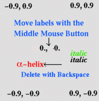
|
The string can be dragged later to any location by the middle mouse button.
The command supports various formats for specifying the label color color_spec and font parameters to characterize the label font font_spec.
Two fonts are at your disposal: the default font (usually times) and the auxiliary
font (usually symbol). Both fonts can be redefined by the
set font
command. You can also switch to the auxiliary font and back inside
the string by backslash-A ( \A). (.e.g "Red: \Aa\A-helix"). You can
also list and delete your string labels by the
list label
and
delete label
commands.
Examples:
display string "Crambin"                            # a simple string

display string "Act.site of \Ab\A-lactamase" yellow # Greek beta letter

build string "ala"
display string Name(a_1.) red 28, 0. 0.9     # first object name
                                             # in the middle
                                             # (font size=28)
display tethers |
display tethers [ as ] [ r_minDeviation ]
displays tethers assigned to the selected atoms as_ with deviation larger than r_minDeviation. Tethers can be imposed between atoms of an ICM-object and atoms belonging to another object, which is static and may be a non-ICM-object. (0. by default).
display volume |
display volume
activates fog from the command line. See also fogStart . Accordingly, the undisplay volume switches the effect off.
display window |
display window [ i_xLeft i_yDown i_xSize i_ySize ]
undisplay window
displays/undisplays the graphics window. When ICM is started without GUI, it is allowed to specify the window size and position.
See also: set window
display window=s_windowList
undisplay window=s_windowList
Displays/undisplays GUI windows and toolbars. s_windowList should be a comma-separated list with ICM panel and toolbar names.
- "opengl" # undisplays the graphics window
- "all" # undisplays all except graphics window
- "alignments"
- "htmls"
- "masterview" # shows/hides workspace panel
- "moledit" # shows/hides molecular editor window
- "plotdialog" # shows plot dialog for the current table (in modal mode)
- "searchwindow" # show/hides chemical search space window. Chemical pattern can be provided optionally as an extra argument
- "columnfilter" # launches column filter dialog for specified table column
- "tablesearch" # launches table "Find and Replace" for the active table. Search string can be provided optionally as an extra argument
- "processes" # shows/hides background job list window
- "prop" # 'Display Panel' with multiple tabs (display/light,...)
- "terminal"
- "tables"
- "moveTools"
- "clipTools"
- "miscTools"
- "viewTools"
- "planeTools"
- "fileTools"
- "selecionTools"
- "tableTools"
You can also display/undisplay individual tabs from the 'Display Panel'. To do that you need to append a tab name to the "prop:".
Example:
undisplay window="prop:light" # hide 'light' tab from the panel
Note: This command does not affect the content of the main working area (the center)
Example:
read binary s_icmhome + "example_search.icb"
display a_
undisplay window="tables" # hides tables
undisplay window="all"    # leaves only 3D graphics window
display window="moledit" Chemical("CCO")  # popups Molecular Editor with compound
display window="searchwindow" Chemical("CC[O;D1]")  # popups Chemical Search Space with compound
display window=s_window center
sets the specified s_window to the center. Windows which may occupy the central position are:
- "opengl"
- "alignments"
- "htmls"
- "tables"
Example:
read binary s_icmhome + "example_search.icb"
display a_
display window="opengl" center # sets graphics window to the center
display window=s_layoutString
Applies the window layout specified in the s_layoutString. ICM stores the layout information as a string in a specific format. Window layout information is stored, for example, in slides.
Example:
read binary s_icmhome + "example_search.icb"
sl = Slide()
display a_
display window=String(sl gui) #changes the view back to what was before the 'display' command
See also: Slide, String slide gui
display GUI windows |
display gui [off] s_window
Obsolete command. See: display window
edit |
edit icmShellVariable
interactively edit the ICM-shell variable using your favorite editor defined by the s_editor variable.
Examples:
   edit mncalls   # actually it is easier to type: mncalls=333
   edit FILTER    # edit a system table, do not change names of components
#
  group table t {1,2,3} "A" {"a","b","c"} "B"  	# create a table
  t						#
  edit t					# edit table t
elseif |
elseif
is one of the ICM flow control statements, used to realize conditional statements. See also: if, then, and endif .
endfor |
endfor
is one of the ICM flow control statements, used to perform a loop in ICM-shell calculations. See also for .
endif |
endif
is one of the ICM flow control statements, used to realize conditional statements. See also if, elseif, and then .
endmacro |
A command ending a macro .
Examples:
   macro threeEssentialsOfLife          # declare new macro
                                        # define essentials
      l_info=no
      modes={"\n\tOoops!!\n","\n\tOuch!!\n","\n\tWow!!\n"}
                                        # randomly pick a line
      print modes[Random(1,3)]
   endmacro
   threeEssentialsOfLife                # invoke macro
Enumeration of charge states |
enumerate charge {chemarray|chemtable} [r_pH=7] [window=r_window(2.)] [name=s_result]
Generates all possible formal charge states at given pH level and window
Enumeration of stereoisomers |
enumerate chiral chem_array [index=I_selectedChems] [center=i_Max_Number_of_Centers] [name=s]
Generates all possible stereo isomers for each chemical compound from
Sometimes you may want to skip compounds with number of unspecified centers greater than certain value. In this case
you should provide center = i_Max_Number_of_Centers argument to the command.
The command will always generate at least one element for each compound.
Example:
enumerate tautomer chem_array [keep] [filter] [index=I_index_array] [name='T_tauto']
The current function only generates tautomers that preserve
the atom content (does not add or remove hydrogens).
With keep option it'll also preserve the hybridization state of each atom (i.e. does not change sp3 to sp2).
Some tautomers are formally possible but chemically do not make much sense.
To avoid generating those tautomers, Split uses the TAUTOFILTER.tab file that
contains the unwanted or chemically impossible tautomer patterns in the SMARTS
format. Feel free to add more patterns to this file.
Use filter option to enable filtering by patterns.
Example file:
enumerate library [simple] chem_scaffold_R1R2 .. chem_R1 chem_R2 .. \
[name= s_libTableName|output= s_fileName] [filter=expression]
Applies chemical arrays (usually a column in a chemical table) for each of replacement groups chem_R1, chem_R2 etc.
to the first element of the scaffold template array. (also known as enumerate library
The scaffold.The scaffold structure needs to be drawn as a Markush structure, e.g.
The replacement groups.Each replacement group in a chemical array (table) needs to have an attachment point specified.
In the Smiles/Smart representation used in ICM it is marked by an asterisk (e.g. "[C*]CC" ).
Marking an atom as an attachment point can also be done in the Chemical Editor ( right-click on an atom and
choose the Attachment Point menu item).
The output table or file.The output table will contain all combinations .
If the output option is specified the resulting library is saved to a file and
the table is not created.
Warning: if the number of combination exceeds 20000 the resulting library is saved to a file
automatically (to avoid memory problems).
The output chemical table has a product column as well as the index of each R-group.
simple option toggle a special mode where instead of full enumeration it simply goes through the input substituents and take i-th element from each.
This mode requires that size of all R-group arrays should be the same. The size of the output will be equal to the size of R-group array(s)
Dynamic filtering of the output by applying a filter expression.The filter= s_expression option allows one to apply a filter during the
library generation. The filter expression is a double-quoted string
with the following structure:
"Function1 relation value & or |
Function2 relation value & or | ..
"
Example:
<>
See also:
A short form of the enumerate library command and linking. The replacement group arrays can be linked to the R positions of a scaffold with
the link group command. In this case a short form of the command can be used, e.g.
Example:
The inverse operation: split the library into scaffold and replacement group arrays.A library can be also reduced back to the scaffold and replacement groups using the split group scaffold library
command. E.g. split group scaffld.mol combilib.mol
See also: make reaction , split group , Replace chemical .
[ Find alignment | Find database | Find database fast | Find molecule | Find chemical | Find pdb | Find prosite | find pattern | Find molcart enumerate | Find molcart | Find table | Find pharmacophore ]
See also: pairwise alignment multiple alignment
find database exact [ distance= i_nOfMutations]] options
find database pattern={ s_pattern | S_patterns } options
find database write [ s_database ]
find database fast [ = i_speed] [output=s_file] [name=s_tabName]
# blast like fast search.
The third version of the command searches for string patterns in a sequence database.
The sequence patterns can contain while cards (e.g. "A?[LIV]?\{3,5\}[!P]").
This search is very fast.
find database fast [ = i_speed] sequence s_dbFile [output=s_file] [name=s_tabName]
very fast dictionary-based sequence search algorithm. Requires a blast-formated database file.
Options:
Example:
See also:
write index sequence command that creates BLAST files from a FASTA file.
[ find-sstructure | find-molecule-sstructure ]
A family of chemical substructure identification commands:
WARNING: This is obsolete way of chemical substructure searching.
Use: find table Index chemical other chemical functions
find molecule reverse ms_1 s_smile
WARNING: This is obsolete way of chemical substructure searching.
Use find chemical instead.
find maximal common substructure in the input set of chemicals.
With the minimize option the command will try to aggregate multiple R-groups into single one (suitable for matched pair analysis)
: find molecule sstructure [ all ] [ tether ] [ hydrogen ]
find maximal common substructure in selected atoms of the two molecules.
Without the all option, one largest pair of matching fragments is identified.
The pairs of equivalent atoms separated by a vertical bar will be stored in S_out, e.g.
Options:
The tether option is useful since once the tethers are established, you can
superimpose a_//T according to these tethers, or optimize the molecule with tethers, e.g.
find molecule [ tether ] as_subFragmentQuery as_IcmTargetContainingQueryFragment
An example:
find chemical ms_sel s_smarts [all]
Searches using smarts pattern s_smarts in ms_sel. The result (matched atoms) will be stored in as_out
With all option it'll find all possible matchings.
Example:
See also:
find molcart enumerate s_space X_patten [stdout|name=s_resultTable] [number=i_maxHits] [nProc=n_parallel]
Efficiently performs substructure search in large (billions) chemical spaces
Arguments:
Example:
find molcart [sstructure|similarity|exact] table=s_molcartTable [ s_smarts|S_smarts|chemarray ] [r_distCutOff] [only] [stereo] [tautomer] [name=s_resultName] [query=s_SQL_condition] [output=s_molcartTable] [number=i_maxHits] [exclude=s_smarts|S_smarts] [append|delete] [ connection_options ]
Performes chemical search in Molcart database.
Connection may be specified by connection_options
Supported search modes are:
Other options:
Examples :
See also: Index chemical Nof Find find table
find table {T_table|filename=<s_file} {sstructure [group]|similarity|exact} [ s_smarts|S_smarts|chemarray ] [r_distCutOff] [only] [stereo] [tautomer] [query=s_ICM_condition] [name=s_resultName|select] [index=I_index]] [append]
Performs chemical and text search in the local table. nProc =
Arguments:
Examples :
See also: Index chemical Find find molcart SMILES/SMARTS other chemical functions
find pharmacophore as_pharmQuery chemarray3D [all]
Performs a pharmacophore search in chemarray3D using as_pharmQuery.
Example:
all option allows one to score all possible mapping for each conformation
See also: Rmsd superimpose makePharma
The simplest parallel script. Note that l_out==yes (or Index(fork)==0 ) defines if the script runs in the parent process.
An example script _multiProc with a hypothetical macro bigDatabaseJob which takes two arguments:
the number of database chunks, the current chunk number, and the output file name:
fork option in for loop
If you have a for loop which performs independent operations on each step you can simple add 'fork
Example:
You can also declare a 'shared' table to pass the data from child process to the parent. Please note that the shared variable can only be of the table type.
For example you have an input table and you want to perform some heavy calculation for each row and put results back into the table:
Example:
Sometime, if the child process can produce more than one (or zero) rows, you can create an empty table in the beginning of
your for loop and append rows during the execution.
For that more you need to add append option.
Example:
Parallel processing with aggregation through the internal pipe and without file output
See also:
- a group of ICM commands with a name and arguments returning a shell data object.
Definition: function name ( arg1 arg2 )
code
code
var = ..
return var
endfunction
Examples:
Example where the function returns a collection
see also macro.
[ group sequence | Group sequence unique | group table | Group column ]
Option pdb activates preferences for higher resolution and first chain names ('a' is better than 'b', etc.)
Option fast will activate the dictionary approach and will give a big time benefit for very large collections (tens of thousand or more).
The comparison criterion is complex and has the following set of preferences which
may be useful in extracting a representative subset of sequences
from a PDB-database:
WARNING: The append option of this function is obsolete. Use add column instead.
create a new table from individual arrays or append new columns or table header elements to an existing table.
This example shows how an ICM table including both header elements and columns may look like:
See also: split, Table , add column (to append columns ) .
For any array type you can apply "concat" operation which will add values into array for each row in the result table
For chemical column "concat_conf" operation can be applied. The result chemical for each group will contain stack of conformation aggregated for that group.
The "uniq" function is the default,
To take values from previously selected "min" or "max" values, use "refmin" or "refmax".
and it means that the unique column values with the same key field will be accumulated
by the group command.
There are two special rules "refmin" and "refmax" which can be applied in conjunction with
"min" and "max" and take rows corresponding to minimum or maximum values in the group.
Note that specifying all option instead of column name will apply operation for all the rest of columns.
Examples:
See also: gui programming
[ Help browser | help | help commands | help functions ]
help command|function|icmVariable|s_icmHelpAncorName
help "I:anchorName"
open the specified section in the ICM Language Reference Manual
help "G:anchorName"
open the specified section in the ICM Program Guide
help s_htmlFileName
# the file name must be followed by the pound sign
opens a single html file in the built-in ICM html browser. This file may contain
sections of icm script in the following format:
help command|function|icmVariable|icmHelpAncorName
For example:
[ Info molcart ]
info auto write
Shows information about when autosaving was performed in the current session.
info molcart [ connection_options ]
Prints additional information about the Molcart connection. Connection may be specified
by connection_options
See also: molcart
Examples:
Note that by default values will be kept only for the one level higher.
With global option changes are propagated through the all nested levels to the global
namespace.
Example :
join [left|right] T1.co1 T2.col2 [ name= s_newTableName ] [ column=S_outputColumns ] [stereo off]
Unites some or all data of the two tables into another table. If the s_newTableName
coincides with the one of the tables, the new table will replace it. The default output table
name is T_join .
The main two arguments are two columns T1.col1 and T2.col2 with matching values.
You can use chemical structure column to join by exact structure match. stereo off option
can be added to ignore chirality.
The column= argument contains the list of column names to be retained in the output table.
Columns in the new output tables.The columns for the output table can be listed as the column=
By default action is to include all columns from both tables.
The columns by which the tables are joined will turn into one, therefore
the total number of columns by default will be N1+N2-1.
Column names of in the joined table.The column takes are preserved unless they collide (i.e. T1.B and T2.B
are both present). The the latter case the first column retains its name while the
column from the second table will be named T2name.colName , (e.g. T_join.B , T_join.T2_B ).
Types of the join commandThere are three types of the join command:
See also the add table ( command for appending a table with identical column structure ) add column or add column function ( adding new columns )
<>
[ Learn atom | Learn chemical ]
learns how to predict column t.Y from other columns or a matrix using the specified method; creates a modelobject.
Options:
type="plsRegression|randomForestRegression|nnKernelRegression|kernelRegression|bayesianClassifier|randomForest|kernelClassifier"
- the training method: partial least squares, principal component regression, kernel regression, nearest neighbor or random forest classifier/regression
kernel="dot"|"polynomial [iOrder C0]"|"radial [exp]"|"tanimoto"|"sigmoid [K C]"
name= s_outputModelName
column= S_columnNames
- an array of column names
all
- forces to use all numerical columns in addition to the chemical column
print={LenMin LenMax nOfDescriptors iType [1:6]}
- chemical fingerprint parameters
test [= nCross|I_excludedTestRows] # cross-validation group number or test rows
center # enforce the constant @@{w,,0} (see below) to be **zero .
select= R_2_c_eps
select= I_LatentVectorSetForPls
unfix
- range normalize the input
this command takes a real array Y and a matrix or table of descriptors
and builds an optimal cross-validated predictive model for property Y.
This command can build several different types of models:
The output of this command is the following:
See also:
Models to predict single atom properties. (e.g: pKa)
learn atom chemarray { R_learnValues|RR_learnValues } print=I_fingerprintParams map=S_atomMappingParams [ exclude=r_correctionThreshold [ number=i_nofCorrectionIterations ] ]
If you have a chemical table which is large enough, say more than a few hundred molecules,
you can build a model to predict a numerical property or binary category of each compound with
Partial Least Squares method (PLS) or Random Forest classifier.
Use this command:
learn propColumn name= ModelName type="plsRegression"|"randomforest"|"randomforestRegression" \
test=n_CrossValidation_Interations \
print= { chainLenMin , chainLenMax , FPsize , binary_vs_count_flag } \
[ map= { atom_map_string, bond_map_string } ]
other_learn_options
This command will take a chemical table and will develop a model. The model can then be applied to
another chemical table using the predict command or Predict function.
Learn Values
Descriptors.
The print argument. The print argument is an array of four integers:
map : Customizing the fingerprint to fit the predicted property
chemical chains of each length can be projected or maped to fingerprints at a different
level of details. This argument has the following structure:
{ "atom_properties_at_lenMin ;
... ;
atom_properties_at_lenMax " ,
"bond_properties_at_lenMin ;
... ;
bond_properties_at_lenMax " }
Each properties section is a comma-separated list of property names:
prop1, prop2, ..;
Example:
Here is the list of possible atom properties.
Here is the list of possible bond properties.
More Examples:
Example:
The information about weights assigned to fragments can be returned by Table function or by Info model function
Example:
Now the final regression can broken down into regression weights, descriptors and regression constant term.
See also: Descriptor , fingerprints , Info model
Multiple linear regression is a statistical method used in data analysis and predictive modeling to examine the relationship between a dependent variable and multiple independent variables. It is an extension of simple linear regression, which deals with the relationship between two variables (one dependent and one independent).
calcMLR M_inputs R_outputs
Example: This example uses a chemical table called XDict and predicts MW using atom counts. Change the name to the name of your chemical spreadsheet.
Artificial Neural Network (ANN) engine can be used to build regression or classifier models. (Special ICM-Pro or ICM-Chemist package is required)
The simplest way to build an ANN model is to use chemical fingerprints or/and set of other numerical descriptors.
In this case building model is similar to the process described in general learn and learn chemical section.
In addition to providing training values and you need to specify the network structure.
learn t.Y type="nnetreg"|"nnet" test=T_cross_valid_set network=C_ANN_structure print=C_FP_parameters number=i_max_training_epochs
Each network layer is defined by collection object with the following attributes:
The final layer (loss function) will automatically be added based on training values type and structure:
Convolutional ANN model takes individual atom properties and chemical graph topology as an input for a training process.
ICM provides number of special operators types to perform convolution operation directly on chemical graph.
This method can be used to train on per-compound, per-atom and per-bond properties.
Two most important layers for chemical convolutional ANNs are:
IMPORTANT: convolutional ANNs usually takes much longer time to train and tune.
learn t.Y type="nnetreg"|"nnet" test=T_cross_valid_set network=C_ANN_structure chemical=s_atomProperties number=i_max_training_epochs
The main difference in learn command to build convolutional ANN is to provide individual atom properties (**chemical= argument) instead
of full chemical fingerprint or descriptors
Atom properties for convolutional ANN
See also:
link g_grob1 [g_grob2 ..] ms_mols_in_one_obj | os_oneObject
The grob can be linked to a molecule, a set of molecules in one object, or to the whole object in order to permit synchronize rotation/translation of those grobs together the linked molecules. The molecules and objects can change coordinates in several operations, e.g. connecting and interactive 3D translations and rotation, or upon superposition of different objects.
The connection mechanism is the following: the selected molecules get a fieldnamed "_GROBLINK_" with the names of the linked grobs.
For example, the icmPocketFinder macro links the predicted pocket grobs to molecules responsible for those pockets.
Example:
link group scaffold i_R_GroupNumber1 chem_array1 i_R_GroupNumber2 chem_array2 ..
associate corresponding Rn positions on a scaffold with the chemical arrays.
This operation copies the chem_array into the scaffold, therefore the external array
which was used to by this command will remain in place.
After the link operation the external array can be deleted.
link group scaffold i_R_GroupNumber delete
delete the association.
link group scaffold i_R_GroupNumber table
link molecule vs_inSeveralIdenticalMolecules
With option molecule , multiple chains of equivalent variables in several
molecules will be formed. Make sure that the variables are properly aligned
and torsion angles are not linked to phase angles.
Examples:
Groups of linked variables can be deleted with the
Arguments and options
Short forms of the command:
Use the ribbonColorStyle="reliability" option and color ribbon
to display the local strength of the alignment.
The strength parameter will be 3D averaged with the selectSphereRadius
radius.
See also:
[ List font ]
list find pattern|word
list font graphic
show currently active fonts used in 2D and 3D labels in the GL graphics window.
The output shows the font number, font size, bold-italic-underline and the number of
labels using this font.
The font number refers to the following fonts:
Example:
See also:
See: Sarray( s_filename_filter directory [ all ] ), sys
list molcart [database=s_dbname]
gives a list of tables in the molcart database.
See also: molcart, rename molcart
list molcart connect
lists all registered database connections.
Note that they do not have to be connected to be listed.
[ Load conf | Load frame | Load molcart | Load solution | Load stack object | Load object ]
load conf os1 i_confNumber [os1_target_for_conf_transfer] [ sstructure ]
Examples:
See also:
load molcart table[=s_sql_table] {T|name=s_result_table} [filter=s_filter] [sort=s_sort_columns] [number=i_limit(1000)>] [ <connection_options ]
Loads rows from a database table s_sql_table.
First i_limit rows sorted by s_sort_columns according to conditions specified in the s_filter condition are loaded.
If some options are not provided in the command and the table
load molcart table T refresh [connection_options]
Reloads requested rows from the database based on the ID values in the primary keys column in
Connection may be specified by connection_options .
If the connection or the table are not specified, this command tries to get their specification from the table header:
Tables produced by the load molcart command are treated as special "database view" tables in the GUI.
See also: molcart, find molcart, query molcart
load stack os [append]
extracts the compressed stack from inside the object and overwrites (or appends)
the existing stack . This mechanism can be used to switch between several
objects withing one session and use their stacks without any need to work with stack files.
Alternatively, in-object-stacks can be saved with the object and read back to a session.
Example:
See also:
Example:
icm_commands
endmacro
To invoke macro just type its name and provide arguments if necessary.
Naming of the formal arguments of macros and functions. The formal arguments in macros and functions need to be named in a special way to imply the type definition.
For example a formal variable which is meant to be a string need to be called s or s_inputstring
Example of a simple macro without arguments:
Example of a shell-function (not to be confused with the built-in functions):
Formal argumentsThe formal argument names should have explicit prefixes
(i_ , r_ , s_ , l_ , p_ , I_ , R_ , S_ , M_ , seq_ , prf_ , ali_ , m_ , g_ , sf_ , as_ , rs_ , ms_ , os_ , vs_ , see above )
to specify their type. The simplest formal argument name is the prefix without the trailing underscore.
If your argument list is incomplete, you will be prompted for the missing argument.
Type q or enter empty string
to quit the macro without execution.
The following features make ICM macros extremely convenient to use:
See also function
[ Make background | Make bond | Make bond multi | Make boundary | make directory | make disulfide bond | Make drestraint | Make factor | Make flat | Make grob map | Make grob from image | make grob matrix | make grob potential | Make grob skin | Make 3d label | make distance | make hbond | make angle | make torsion | Make image | Make key | make map | make map cell | Make map factor | Make map potential | make molcart | SAR analysis | R-group decomposition | make pca | make peptide bond | Make map xray | Make plot | Make reaction | Make sequence alignment | Make sequence | Make sequence random | make tree | make tree object | Make unique ]
make background s_external cmds [command=s_icmCmdsUponCompletion] [info=s_Message] [name=s_jobName] [simple]
This command runs a set of external commands written in a form that can be executed
as an external process. Upon execution of these external commands the ICM client will
receive the s_Message ( by default it will be the following message:
"background job 'jobName' completed. Press OK to load the results".
You can also specify which commands can be executed by the ICM client to load
the results of this job.
Arguments:
The make background command the following features:
simple option creates completely detached job. ICM will not keep any information about that process.
This option is useful if you want simply to launch an external program and don't want to have any further
interaction with it.
See also:
adds a covalent bond between two selected atoms in a non-ICM molecular
object (e.g. X-ray or NMR pdb-entries) or resets the bond type (for ICM objects use make bond simple
The command is used to correct
erroneous connectivity guessed by the read pdb command.
This correction makes the molecule displayed in the graphics window look
better and is necessary before conversion into an ICM molecular library entry
(see icm.res or user library files) using the write library
command.
It can also be useful to display a connected Ca-trace.
In interactive graphics mode you may type make bond
and then click two atoms with the Control button pressed.
make bond simple as_singleIcmAtom1 as_singleIcmAtom2
forms a bond, e.g. for peptide cyclization. One needs to unfix the following energy terms for
that bond to be minimized properly:
make directory s_Directory
Examples:
make flat chem_array [rotate] [hydrogen] [window=r_WidthToHeightRatio] [index=I_indices] [pattern=X_scaffold]
convert a chemical array into standard automatically generated 2D chemical drawings in place
(compare with Chemical( Smiles( chem_array ), smiles ) which does not touch the source array).
A chemical array can created by the read table mol command.
The compounds in the source file can be 0D (all coordinates set to 0), 3D or 2D.
In all cases these x and y coordinates are can not be used for chemical drawing and
one needs to use the above command to generate 2D drawings.
The command also preforms rotation for optimal fit into rectangle with specified width to height ratio ( window argument ).
Default ratio is 1.5.
Other options:
Example:
make grob m_map add r_sigmaIncrement
make grob m_map add exact r_absoluteIncrement
# build a contour that can be modified
make grob g_existingContourGrob add r_sigmaIncrement
# rebuilds and redraws an existing contour
Create graphics object by contouring electron density map at a given threshold.
threshold: By default the contouring level is calculated as the mean map value (returned
by Mean ( m_map ) ) plus mapSigmaLevel times root-mean-square deviation value.
If a real value argument is provided, the mapSigmaLevel shell variable is redefined.
Option exact allows one to specify absolute value at the contouring is performed.
If atom selection is specified, contour will only be built around as_, with the optional additional margin. Helpful in contouring ligand from electron density map.
The grob can be 'link-grob{linked} to a set of molecules in one object, or to the whole object to
change coordinates in 3D the grobs together the those molecules upon connecting and interactive 3D translations and rotation, or upon superposition.
Other options:
Example:
make grob surface [color] [wire | smooth] [as_1 [as_2]] [[name=]s_grobName] [r_transparency]
See also: set color to set atom colors
A number of commands in ICM enable the creation of "3D label" objects which help to measure and annotate geometry in the 3D space,
like distances and angles. Some 3D labels, like hydriogen bonds, illustrate concepts which depend on the geometry
and the structure of molecules.
3D labels are stored in a parray object of a "label3d" subtype.
3D labels defined on atoms are dynamic: visual angle/distance information is updated depending
on the changes in the atom geometry.
3D label creation commands have similar structure.
Commands which are currently available are:
Each of these commands has specific arguments. but there is a number of common options:
creates a parray with distances between all atoms in as_1 and as_2,
or all atoms within as_1 if the second selection is not specified.
Output
Examples:
Example in which we detect clashes:
See also:
creates an array with all hydrogen bonds contained in as_1, or between as_1 and as_2 if the second selection is specified.
Hydrogen bonds are calculated according to several shell parameters listed below.
It is possible to specify the upper limit for the distances between atoms which will be considered as potential bond
using the r_maxdist value.
Other options and shell parameters:
See also:
creates a planar angle 3d label. Requires a selection containing 3 connecting atoms.
See also: make 3d label , Table(angles,distance)
creates a dihedral angle 3d label. Requires a selection containing 4 connecting atoms.
Examples:
See also: make 3d label , Table(tors, distance) .
make image [library=s_albumName] name="Party2007.png"
will save the graphical image to the internal album (a parray ).
The name will be used if you decide to save the album to a file.
Example:
This command generates a binary chemical key, i.e. a bit-string in which each bit corresponds to
a chemical substructure, converts the bit-mask into
the hexadecimal string and saves this hex-string in s_out .
The bit-string with chemical substructure information can then be
used to calculate the Tanimoto similarity distance with another chemical key.
A family of commands producing maps. It includes:
make map potential [simple|occupancy] [s_terms | name=s_mapname] [as] {[R_6box] [r_gridCellSize] | cell=map } [ l_ecep=no|yes ]
The default map (with no terms provided) will return an electron density map. It supports the occupancy argument as well.
Each individual term (say, "gp") may result in creation of one or several (up to seven)
different grid maps. These are the maps created under different terms:
See also:
make map potential m_electronDensity to generate a rectangular grid from
an oblique crystallographic density map.
make molcart table T name=s_dbtable [ make_options] [ connection_options ]
Imports data from ICM table T_ into database table s_dbtable.
make molcart table s_filename [ mol | smiles | separator [header] ] name=s_dbtable [ make_options] [ connection_options ]
Imports data from the s_filename file into database table s_dbtable.
The file format may be guessed from the s_filename or specified explicitly. Supported formats are:
Connection may be specified by connection_options .
Other options ( make_options ) available:
make molcart table input=<[s_connectionID;][s_db.]s_sourceTable> name=<[s_db].s_targetTable> [append] column=S_column_specs connection_options
Copies data from one molcart table to another.
Example:
See also: molcart, write molcart.
make molsar {T_chemicalTable|X_chemicalArray} X_scaffold [auto] [append] [name=s_ResultTable>]
Performs R-group decomposition using X_scaffold. This command is similar to split group command.
The only difference is that single table will be generates. For each R-group in the X_scaffold a column
will be created.
With append option the original compound will be added to the result table.
With auto option no explicit R-group specification is needed. The command will automatically find
attachment positions and create appropriate columns. Columns which are invariant (no changes in substituent)
will be excluded.
Example:
See also: split group , split-groupenumerate-library , make reaction , Replace chemical , Find chemical
split molsar {T_chemRgroupTable|R1_col R2_col} [R_propColumn1 R_propColumn2 ...] [name=s_sarTable] [color=R_] [rainbow=s_rainbow]
generates one or more 2D SAR analysis tables from the input R-group columns.
make pca [append] T [i_nPC=3] [r_tradeoff=0.010000] [options]
Options:
Note that this method uses distance constraints (as it is done for the disulfide bonds) to support the closure.
Another method:
make map potential map_Xray [as] [R_6box] [r_gridCellSize] [smooth] [name=s]
converting crystallographic density map which is not suitable for energy manipulations
to a grid potential m_xr . The source map starts at {0.,0.,0.}, can be oblique with uneven spacing.
However the resulting map is always equally spaced rectangular map in any area of space.
This grid potential can be used in real space refinement.
Find the description of the arguments in make map potential command.
Option smooth uses the Gaussian smoothing of the values.
See also:
make plot T s_plotArgs [name=s_plotname [append]] # GUI, interactive plot in an open ICM session
make plot T s_plotArgs [output=s_fileName [window={i_w,i_h}]] # generate and save the image to file
This command creates a plot belonging to table T . The first one will create a plot in your open ICM session next to a table, of your choice, while the output= and window= options result in creating this plot and directly saving it as an image to a file.
Each table can contain multiple plots and all the plots created interactively belong to the following sarray of the table header: T.plot, e.g. T.plot[1] . Note that it is an array because the same table may have multiple plots associated with it.
One can actually build a plot interactively, then look up T.plot[1] save it, and use as a template of as regeneration of the plot from command line.
The s_plotArgs string contains the arguments, e.g.
The syntax of the s_descr string containing other arguments of the make plot command
is the following.
plot_element[;;plot_element2;;...][general_plot_properties]
Plot elements.Each double-semicolon separated section is either a plot/histogram or a geometrical element.
Histogram plot arguments
The syntax of the columnName can refer to one or multiple columns as follows:
columnName|{columnName[,columnName...]}
A distinct columnName can be further split by another columnName as such:
columnName[:columnName]
Examples:
General Properties (all are optional, and added at the end after )All general properties are added at the end of the plot string, with each argument separated by two semicolons (;;), e.g. make plot
Properties of the geometrical elements (rectangle,ellipse and polygon)
Example
Option output writes the plot as an image into file name provided. File extension defines the image type.
(Most popular extensions: png,jpg,pdf,eps)
With output option you may additionally specify the size of the output image.
Example:
Visualizing a matrix
Element matrix=matrixName with additional arguments:
See also:
make reaction reaction_R1R2 chem_R1 chem_R2 .. [name=s_table | output=s_file] [filter=s_expression] [all | only ] [ keep ]
Takes one chemical reaction (the first element of a reaction array) and applies it to
the reactant arrays. All reactants suitable for this reaction will be combined to generate
a chemical table .
The reaction drawing need to refer to replacement groups as R1 , R2 , for example:
keep options preserves SMARTS search attributes in the result
all and only options allows one to handle multiple functional group mapping. The possibilities are:
You can apply a filter expression to the output of the reaction. The following functions can be used
in the filter:
MolWeight,Nof_Molecules,Nof_Chirals,Nof_RotB,Nof_HBA,Nof_HBD,Nof_Atoms,Nof_Frags,MolSynth,MolLogP,Volume,MolPSA,MoldHf,MolLogS
Example:
You can also apply condidtion to the matched functional groups. R1,R2,...
Example:
Another example (provided as an example file):
The output. The output is generates as a table if the total number of products is less than 40,000.
For larger sets the command will automatically switch to the file mode.
The output chemical table has the product column as well as a column for each of the R-groups.
Dynamic filtering of the output by applying a filter expression.The filter= s_expression option allows one to apply a filter during the
library generation. The filter expression is a double-quoted string
with the following structure:
"Function1 relation value & or |
Function2 relation value & or | ..
"
Example:
The list of functions is expanding. The current list of the functions is here
Splitting the library by the scaffold into the replacement group arrays.A library can be also reduced back to the scaffold and replacement groups using the split group scaffold library
command. E.g. split group scaffld.mol combilib.mol
See also: enumerate library , Split chemical , Replace chemical .
make sequence ali_range
make sequence ms [name={s_name | S_names}] [resolution]
make sequence nSeq [ lenMin [ lenMax ] ] [name= s_nameRoot ('sq') ]
generates nSeq random sequences with length randing from lenMin to lenMaxExamples:
make tree table [tree_type] [tree_name] [options]
this command builds a hierarchical data tree of the table rows and stores in the table header.
as a tree.cluster parray.
A simple example is given below:
Defining the tree construction type.
The main modes are the following:
For a small number of rows ( N under two thousands)
ICM performs data clustering based on N by N comparison between the table rows.
This method can be enforced for larger tables with the full option (e.g. make tree t full)
or using the distance = s_distMatrixName . In the latter case the matrix needs to be appended to the
table header:
The type ( tree_type ) of the cluster tree construction algorithm can also be explicitly defined.
This type defines how two distances from two neighboring branches are replaced with one distance.
By default the "upgma" method is used.
If the number of rows N is large, ICM performs the K-means clustering by default. The K-means method can
also be enforced if the number of clusters is provided as an explicit integer argument, e.g.
Defining the distance measure.
The distances between rows can be (1) provided externally in the table header
(option distance=s_matrixName, see below )
(2) calculated dynamically as Tanimoto distances between chemical fingerprints for chemical tables;
(3) calculated dynamically as weighted cartesian distances (options column= S_listOfColumns
and heavy= R_listOfColumnWeights ).
The tree can further be used to assign a cluster number to each table row at
a certain distance threshold ( the separator= and the split= options ).
For common tables, by default all numerical tables are used with the same weight.
For chemical tables, by default only the chemical array is used for distance calculations.
However, option all will enforce concurrent use of the chemical distances and all numerical columns.
Options column= and heavy= give a specific selection of columns and their respective weight.
The output.
Example:
make tree ali_name [ s_epsFile ]
make tree object M_dist_nxn [S_names_n] [name=s_objName] [angle=(90:180)] [torsion=(0:180)] [simple] [size=r_distScale]
makes a 2D (option simple ) or 3D tree and sets an integer field named 'index' with
the index value to each atom (see set field and Field( as s_fieldName ) )
This example shows how to start from a table and make an active tree (nodes respond to doubleClick) :
[ Minimize cartesian | Minimize loop | Minimize stack | Minimize tether ]
minimize cartesian|mmff [type] [charge] .. \n\
minimize stack [selftether] .. \n\
minimize tether [disulfide] .. \n\
stack :
If option stack is specified, the procedure extracts each stack conformation,
minimizes it and replace the stack conformation with the optimized ones.
The stack can be generated with the montecarlo procedure, manually created
with the store conf command, or read from a stack file.
This command allows one to refine your set of alternative conformations all at once.
atom pair filter:
By default all the atoms and all the atom pairs within distance thresholds vwCutoff and hbCutoff
are involved in the calculation.
However, two explicit atom selections [ as_1 [ as_2 ]] may
impose a mask on atom pairs involved in the calculation of the pairwise energy or penalty terms.
The default for the skipped as_1 is all the atoms.
If only the as_1 is specified, the as_2 is assumed to be all atoms.
Using atom selections is dangerous and is not recommended since there are many
combinations which do not make sense and give unpredictable results.
Suppressing updates of the interaction lists upon atom movements during the minimization. Sometimes during the course of minimization the interaction lists are recalculated.
When some atoms fall out or in the vwCutoff sphere , the value of the gradient and even the energy function
can jump. For that reason do not be surprised that the exit gradient differs from the one reported in the previous
step output. To influence the lists you have two main mechanisms:
The minimizer also returns a rarray R_out with the following values:
minimize cartesian [simple] [stack] [type] [charge] [i_mncalls] [s_termString] [selftether=as_for_ts_term]
Assigning ring conformation from a template
To assign ring conformation from a template one can use the minimize tether command.
The chemical equivalences can be found and tethers imposed with the find molecule sstructure all tether command.
The following example illustrates the principle.
modify chemical structure of a molecule by replacing one part with
a specified group or "residue" from icm.res or user residue library.
Prerequisites:
replace selected residue(s) rs_ by another residue s_NewResidueName.
The backbone conformation is not changed, unless the new residue is "pro" and the phi angle
is outside [-90.,-30.] range.
Examples:
Modifying the 1st residue in a polypeptide
The first residues has an unusual N-terminus therefore there is a special trick to mutate it to another residue.
Essentially the grafting principle (see below) needs to be used.
Example in which we are modifying 1st residue of the first object:
Note: consider using macro modifyGroupSmiles as_replacement_atom s_chemsmiles
to avoid side effects of the straight modify command.
This macro makes sure that your branch does not start from the first atom and minimizes the connection afterwards.
See also: chemical modification of chemical arrays
modify rotate [os_nonICM] [i_n_perm(1)] [only]
performs one or two (if i_n_perm is 2) circular permutation of Cartesian coordinates of atoms and unit cell parameters
a,b,c and alpha,beta,gamma parameters of the unit cell.
Example:
[ Chemical Find and Replace | Modify chem charge | Modify chem delete salt | Modify chem normalize | Modify molcart ]
find and replace a chemical pattern, normalize/standardize a chemical, delete salts
The following types of chemical modifications can be performed on an array of chemicals:
modify chemarray s_find_smart s_replacement_smart [exact] [ index= I_indices ]
find a chemical pattern and performs a global replace to s_replacement_smart for all chemicals in an array.
The replacement can be done only if both the find and replace patterns contain the same marks R1,R2..
A connecting atom in the pattern can be either an undefined atom, e.g. [R1] or a defined atom, e.g. [C;R1]These marks are used to find corresponding atoms in the replacement pattern.
Hints for the Chemical Editor: use the following shortkeys:
E.g:
modify chemarray s_find_smart s_replacement_smart [exact] [ index= I_indices ]
searches for a chemical group and replaces it by a group with a different charge.
Add index= I_idx if you want to apply the operation to a selection.
Carboxylic_Acids
modify chem "CC(=O)[O;D1]" "CC(=O)[O-]" exact # to charge
modify chem "CC(=O)[O-;D1]" "CC(=O)[O]" exact # to uncharge
Primary_Aliphatic_Amines
modify chem "[C;^3][N;D1]" "C[N+]" exact # to charge
modify chem "[C;^3][N+;D1]" "C[N]" exact # to uncharge
Secondary_Aliphatic_Amines
modify chem "[C;^3][N;D2][C;^3]" "C[N+]C" exact # to charge
modify chem "[C;^3][N+;D2][C;^3]" "C[N]C" exact # to uncharge
Tertiary_Aliphatic_Amines
modify chem "[C;^3][N;D3]([C;^3])[C;^3]" "C[N+](C)C" exact # to charge
modify chem "[C;^3][N+;D3]([C;^3])[C;^3]" "C[N](C)C" exact # to uncharge
Amidinium/Guanidinium
modify chem "[N;D1]C=[N;D1]" "NC=[N+]" exact # to charge
modify chem "[N;D1]C=[N+;D1]" "NC=[N]" exact # to uncharge
#
modify chemarray {delete|split} salt[ = chemarrayWithSalts [add] ] [simple]
Removes salts using dictionary file $ICMHOME/SALTDICT.sdf.
Since salts may contain multiple instances of the drug (e.g. Drug.Ca.Drug ) additional cleaning may be needed
Option simple just considers will just leave only the first molecule.
Example:
New or additional salt patterns can be provided with salt=.
Example:
with add option both default and used provided dictionary will be used.
split option created two new columns in the original table 'salt_smiles' and 'salt_names' with dot separated smiles and names for removed salt.
simple option toggles mode which retains only the largest molecule and deletes all smaller molecules.
Example:
modify chem_array auto
applies a set of chemical normalization rules described in the CHEMNORMRULES.tab in the $ICMHOME directory .
Feel free to add rules to this table or replace it with your own table.
Currently it has the following rules:
See also:
modify molcart T [all] [column=S_columns] [table=s_table_name] [ connection_options ]
Modifies entries in a database table based on changes made in an ICM table.
The load molcart, find molcart and query molcart create ICM tables containing subsets of database tables.
In most cases the database table has an integer primary key (ID) column, with unique values for each row.
The primary keys may be used to mark certain rows in the ICM table to request update or deletion of the corresponding
entries in the database. ICM GUI provides tools to mark rows.
The all option tells the command to treat all rows as marked for update.
Only a subset of the ICM table columns may be updated in the database by specifying S_columns.
The connection may be specified using connection_options . Database table is specified
Otherwise connection and table information may be obtained from the input table header as in the load molcart command.
See also: molcart.
[ montecarlo-fast ]
montecarlo [ OPTIONS ] [ vs_MC [ vs_minimize ] ] [ local rs_loop ]
tautomer
toggles tautomer sampling. (`build-tautomer needs to be called before)
fast :
bfactor :
option store means that at the end of the simulation the stack is stored in
the current object (equivalent to the store stack object command ). This allows
to extract it later without reading it from a file.
superimpose as_3atoms_per_molecule
trajectory [ Move molecule | Move object | Move bonding | Move element | Move column | Move plane | Move sequence ]
move os_ObjectToMove os_destination
move ms_molecules_to_merge [ s_new_mol_name ]
move only ms_molecules_to_merge
different molecules in a PDB object can be merged into a single molecule and correct intermolecular bonds can be formed with this command.
This command also automatically
bonds the closest atoms (if distance< 0.6(R1+R2) ) between the molecules being merged into a single molecules.
Helpful in dealing with PDBs with disconnected carbohydrates.
Options:
Example;
move table[i_row] [i_newPos]
moves a row, e.g. t[2] to a new position.
If the position is not specified the row is moved to the end.
move parray[i_pos] [i_newPos]
moves a parray element to a different position.
Example:
move table.column [ i_newPos ]
moves the column to a new position. If the position is not specified the column is moved to the last position.
Example:
See also: add column, add column function
move plane r_ofs [all|reverse]
command line interface to clipping planes
Arguments:
Example:
move ali seq [i_new_seq_pos]
move the sequence in an alignment to a new position. If the position is not specified, the sequence is moved to the last position.
Example:
[ debugger ]
See also the make plot associated plot method, for example
predict model T_n [ M_nxm ] [key] [ name= s_colName ]
command applying a model developed by the learn command.
It is printed to stdout . To print to stderr use the printf error ... command.
print bar { "." | " Start" | "End\n" } nSteps
Useful in showing progress in a long for loop.
Example:
query molcart s_sql_command|S_sql_commands [name=s_tableName] [connection_options]
Performs an SQL query in the connection specified by connection_options .
For SELECT and other queries returning data, this command creates a table.
The result table may be specified by the s_tableName parameter.
All SQL types are converted to appropriate ICM types.
Example:
See also: molcart, find molcart, load molcart
[ Randomize angles ]
[ read from file | Read binary | Read gui | Read html | Read fromstring | Read with filter | read all | Read index table | read http/ftp | read unix | read unix cat | read alignment | read color | Readcomp_matrix | Read conf | read csd | read database | read drestraint | read drestraint type | read factor | Read gamess | read grob | read iarray | read index | read library | Read librarymmff | read map | read matrix | read mol | read mol2 | read trajectory | read object | read pdb | read pdb sequence | read profile | read prosite | read rarray | read blob | read sarray | Read file by chunk | read sequence | read stack | read string | Read table | Read table chunk | Read smiles | Read table html | Read table mmcif | Read table mol2 | Read table mol | Read column | Read variable | Read view | Readv restraint | Read vrestraint type | Read xml | Read json ]
Option pattern = regexp will filter out the lines of the text file that match the regular expression.
[ read-binary-list ]
read binary pdb s_pdb_code
# see also s_xpdbDir
Reading everything or just some itemsBy default, ICM reads all objects in the file. If you want to see
the list the objects in this archive, use the list binary command.
To read selectively, use the name option or a list of object classes, e.g.
Options:
creates a table of content for the icm objects stored in a binary file.
It the table name is not specified, T_out table is created.
From the GUI interface you can double click on a table row to download a
particular object from the file.
From a command line one can read the desired objects with read binary file name= s_names or S_names
read gui s_gui_filename
read a file with menus to modify, update, or extend the existing ICM menus.
The format of the menu file is described in the gui programming section.
You may also find many examples in the $icmhome/icm.gui file.
Example:
read html [ display | auto ] s_htmlFile [ name= s_newStringName ]
read an html file and display its contents in the built-in ICM html-browser.
This command also creates a string variable.
Options:
If a html-document is read to ICM with this command, it can be stored in a single project along with
other objects of the ICM shell.
read html simple s_htmlFile
does not create a shell variable, just displays the file with txdoc .
The HTML documents can contain sections of the icm code (so called icmscript ) which
are executed upon clicking. Example:
See also: help browser .
read ... s_compressed_or_encoded_files
Example:
See also:
read .. "ftp://ftp.server.com/path/to/file"
reading directly from ftp port.
The ICM can read not only from files directly accessible from your computer but also files from
remote locations via ftp or http.
ICM includes a simple FTP client to simplify access to the
databases on the internet.
Files names may be specified as an ftp style URL:
read .. "http://www.server.com/path/to/file"
reading directly from http port.
ICM includes a simple HTTP client to simplify access to the
databases on the internet.
Files names may be specified as an http style URL:
Example:
You may pass arguments to the http URL using POST or GET methods.
See also: HTTP.proxy FTP.proxy
read gamess s_gamessOutputFile
reads and parses the output of the gamess program. ICM converts the atomic (Hartree) energy units into kcal/mole
and with some options can upload the minimized conformation.
read grob s_groFileNameRoot [name=s_grobname]
See also: write grob .
read library [ s_libraryFileNameRoot ]
read library [ residue | atom | color | drestraint | vrestraint | charge | energy ] [ s_libraryFileNameRoot ]
Conformational generationThe _confGen script creates a table called conformers. In this table multiple conformations
of the same molecule can be recognized by column MOL_NUM with the molecular number in the input file.
Now the multiple conformation can be read into a molecular object with a stack like this:
Some properties of the current object a_ which can be extracted (most of them are
also applicable to any selection):
read object parray s_obfile [name=svarName]
reads objects from .ob file into a parray . In this case the objects are not loaded into the
workspace but instead are stored in an array. The array can also be added to a table, e.g.
[ read-pdb-mmtf ]
read pdb [all [stack]|charge|delete|header|html|sstructure] [ s_pdbFileNameRoot [ .mol/res1:res2/at1,at2,..] ]
read pdb-formatted file and create a molecular object of a corresponding.
You can read all the information from the file or only the part you need:
See also:
read binary pdb
read pdb mmtf s_pdbCodeOrFileName
reads PDB entry in MMTF format. MMTF is a compact binary format which is particularly
useful to read large PDB entries which cannot be represented in standard PDB file format.
Example:
The number of residues which are present in the SEQRES record, but are missing from
the ATOM records is returned by the i_out variable, or Field( a_ 15 ) function.
read blob [ s_fileName_or_URL ] [ name=s_blobVar ]
read any data from ~s_fileName_or_URL or standard input into blob shell variable.
Options:
read sarray [limit=n_records] [keep] [separator=s_sep] [ s_fileName ] [ name = s_varName ]
reads up to n_records. s_sep is used as a record separator.
Sets l_out to yes if the end of the file is reached.
keep option keeps file open for the next read chunk. Without keep the command will always read from the beginning of the file.
Example: (read uniprot file)
Example:
Option auto (with fasta or pir) will create an alignment if all sequences (with dashes) in a multiple fasta file have the same lengths.
Option selection (with fasta or pir) will create a selection if the sequences read.
read sequence swiss [full] [ field= S ] [ group [= s_groupName]] [ s_seqFile ]
read sequence swiss [full] web s_swissProtName
With option swiss i_2out contains the next residue after the signal peptide or 1 if no signal is found.
Option full will read all FT sites with their full description.
See also Table( seq_swiss site ) function.
Example:
Note,
that if you want to ignore some types of the swissprot FT feature table, e.g.
HELIX, or COIL, see swissFields )
s_fieldDelimiter is NOT used in the ICM table reader. If you want to change the default field delimiter use the
split= s_fieldDelimiter argument. To skip multiple occurrences of a delimiter symbol, repeat it two times, e.g.
split= " \t\t" ( the same trick is used in the s_fieldDelimiter variable for the Field function )
read table separator=[","|"\t"|":"|"$"..] s_csvtableFileName [delete][header][simple] [name=s_tableName] [comment= s]
reads tables in portable csv (comma-separated-value), tsv (tab-separated-value) or other separator-based text spreadsheet formats that can be exported from excel.
Options:
Flanking blanks for each field are trimmed. For example to read the following table from iq.csv file:
read table sv_file separator= s_symbol name=s_tabname keep limit=i_nRows
reads from a large table a chunk or rows.
Here is an example how to read a file without column headers
See also:
read smiles [header] s_filename [name=s_newTableName]
reads the s_filename file in smiles format into a table. Table name is derived from the file name
if s_newTableName is not specified explicitly.
With the header option specified, the first line in the file is used for table column names.
Example of the space-separated smiles file with header:
read table html s_htmlFile|or URL [name=s_newTableName] [all] [header=[yes|no]] [simple]
this command will read a file containing one or several html tables,
then will select the largest table (by the number of rows) and read it into an ICM table.
Options:
read table mmcif s_mmcifFile
reads a pdb mmcif file with multiple small molecules (not for the whole pdb)
into a chemical table. The short description of mmcif format is given below.
The full description is provided by pdb .
This command will create a chemical table and all general properties will be converted into columns.
Example (reading all PDB ligands):
read table mol2 s_mol2FileName
reads an mol2 file into an ICM table which can be visualized as a chemical
spreadsheet.
read table mol [ exact | unique ] [simple|simple=S_cols] s_sdfFileName [ index ] [limit=i [keep]]
read table mol [ exact | unique ] T_sdfFileIndexExpression [ index ]
The table name is saved to the s_out variable.
The property fields of the sdf file, e.g.
Reading chunks from t.sdf and spitting out chunks of the itb stream:
Another way to read a table into ICM arrays is to read it as table with the read table
command and split the table afterwards.
read XML formated document into a hash(formely collection ) object.
read xml { s_fileName | s_url | input=s_xmlBuffer } [name=s_name]
Example:
See also: array , xml drugbank example
JSON (an acronym for JavaScript Object Notation pronounced) is a lightweight text-based open standard
designed for human-readable data interchange. Read more here.
read JSON formated document into collection object.
read json { s_fileName | s_url | input=s_jsonBuffer } [name=s_name]
Example:
[ Rename column table | Rename molcart | Rename system | restore preference ]
rename atom as1 s_newElement\n\
rename column table ...
rename as1|rs1|ms1|os1 s_newName # rename os full -for description\n\
rename image P_imageArray i_index s_name\n\
rename page P_pageArray i_index s_name # see below, for icmdb\n\
rename sequence resolution # from 1abc_a to 1abc_a21 for sequences linked to a_A. used in group unique..\n\
rename anything to anything else. More specifically you can rename
commands, ICM-shell variables, objects, molecules, residues and
atoms. Renaming commands is possible, but then you must not forget to
change them in all the standard ICM-scripts. Using aliases
instead allows you to use both the original and the translation,
however it slows down the ICM-shell interpretation. Be careful with
a new name to avoid name conflict.
rename column tab [column selection [inverse]] [name=S_new|s_colname_base ("A")]
renames large groups of columns, handy for table with thousands of columns, a good method to simplify and shorten column names. Allows to create excel style names or names reflecting column index (e.g. t.1 t.2 t.3 ... )
Arguments: column_selection: There are multiple ways to specifiy columns to be renamed (option inverse inverts the selection ):
Destination namesThe destination names are specified either by a string array of new names (with or without the table name)
under the name= option (e.g. name="A"//"C"//"Name" ) , or by a string with the root name of the first column to be renamed
( e.g. "A", or "1" )
See also: rename, delete column table, select column table
>>rename-object{rename.molecule,rename.residue,rename.atom}
h4-- rename object
rename { os [ full ] | ms | rs | as } s_newName
If you rename multiple molecules and provide a s_neweNameRoot (say, "a") at attempt will be
made to name them like this: "a","a1","a2",... .
Groups of atoms also can be renamed from a chemical (2D) template with the
set bond topology as chem_source label command.
rename molcart table s_oldTableName s_newTanbeName [connection_options]
renames Molcart table including all index tables.
Database connection may be specified by connection_options
The table name s_oldTableName may be prefixed by the database name, else current database is assumed.
See also: molcart, list molcart
rename system s_fileNameFrom s_fileNameTo
Renames or moves a file. If target file exists it will be overwritten.
Example:
See also: sys , delete file delete directory
restore preference [ all | prefname1 prefname2 ... ]
restores values of the named (or all) GUI preferences to the default values.
[ rotate object | rotate grob | rotate view | rotate chem ]
Also, to perform a fixed number of interruptible rotations or rocking movements, use this:
See also: interruptible background rotations and rocking movements.
rotate the 2D depiction of chemical structures in a .mol column of a table
of a chemical compounds.
[ Select chemical | Select column table | select-3d-label ]
The main select commands:
select [off] [alignment | grob|iarray|map| matrix| profile| rarray| sarray| sequence| table..] [s_namePattern]
(un)selects ICM objects with certain name pattern (or all), e.g. select grob "g_pocket*"
select chemical ...
select patterns in 2D chemicals of a chemical table
select alignment as
select [dist|distance|hbond] as
select treeArray center
See also:
This command can be used for:
Align 2D chemical by pattern ( with rotate option )
select chemical chemarray {s_smarts|chempattern} rotate [index=i|I]
Select matched fragments(s) ( with all and/or append option)
select chemical chemarray {s_smarts|chem} [all] [append]
Color matched fragments ( with color option)
select chemical chemarray {s_smarts|chem} color=s_color [all] [append]
Use atom-level predicate s_filter to color/select individual atoms.
select chemical chemarray filter=s_filter [append] [color=s_color]
s_filter should contain a logical expression which may use certain atom-level properties.
Examples:
See also: delete chemical selection find table
select column tab [only] [column selection [inverse]]
selects large groups of columns in GUI, handy for table with thousands of columns, helps to avoid excessive painful clicking.
Arguments and Options:
column_selection:
See also: delete column table, rename column table
select [edit] 3d-label
graphically selects the specified label. It appears as a little green cross. The labels are considered as a subclass of
graphical objects.
Options:
See also:
[ Set area | Set atom ball label | set atom | Set background image | set bfactor | set bond type | Set bond topology | Set cartesian | Set chain | set charge | set charge formal | set charge formal auto | Set chargemmff | set chiral | set chiral chemical | Set color | set comment | Set alternative atom | Set comment sequence | Setcomp_matrix | set directory | set drestraint | set drestraint type | set group column | Set hydrogen | set site | set site alignment | copy site | Set site residue | set slide | set tautomer | set texture | set error | Set field | Set field alignment | Set field map | Set field name | set font | Set font grob | Set foreground | Set format | Set grob | set key | set label | Set map | Set molcart | Set name | Set object | set occupancy | set plane | set pmf | set property | Set property column | set chemical view options | Set property alignment | Set randomize | set resolution | set stereo | set sstructure backbone | Set sstructure sequence | Set stack | set swiss | Set symmetry crystal | Set symmetry bio | Set symmetry | set table | Set terms | set selftether | set tether | Set tether append | Set type | Set type surface | Set type property | set object type | set molecule type | set type sequence | set type mmff | Set vwradii | Set vwelradii | Set view | set vrestraint | Set vrestraintvs_var | Setvs_var | Set variablegrid | Set window | Set xstick ]
set area|atom ball|as ..|background|ball|bfactor|bond|cartesian|chain|charge|chiral|color|comment|comp_matrix|
conf|
directory|drestraint|edit|error|factor|field|font|foreground|formal|format|grob|group|header|hydrogen|
index|key|label|link|map|menu|mmff|molcart|name|object|occupancy|plane|property .. |randomize|
reflection|resolution|selftether|separator|sequence reverse|site|slide|sstructure|stack|stereo|stick|swiss|symmetry|
table|tautomer|term|tether|texture|topology|torsion|tree|type|view arguments
Example:
set atom ball as R
sets custom balls to atoms. Can be returned with the Radius( as ) function
set atom label as S
sets custom labels to atoms. Can be returned with the Label( as ) function
(re)sets atom properties, such as atom presence ( on and off ) or coordinates
set as on|off
activate (unhide) or inactivate (hide) atoms for energy and surface calculations.
The inactive atoms can be shown in
graphics as shaded wire models. Example: set a_//h* off ; Nof(a_// off) ; set a_//h* on
By default all atoms are active. If a selection of atoms in 'off' or inactive, this state may also be added to the object stack with the store conf atom obj_sel command. Be careful since the very first conf should also be added with the store conf atom .. command for this mechanism to work.
See also: Nof(
set as_Natoms M_3xN [mute]
set as_tethered_inICMobj [tree]
# follows tethers in this case the target coordinates are simply taken from the destination positions for the tethers.
set as_one_vt1_atom_inICMobj [R_3xyz|M_3x1|as]
set as_nonICM_X as_ICMtetheredToX
# used to update sdf/mol coordinates after optimization.
this command is used to inherit the coordinate changes in a converted object with different order of heavy atoms.
Imagine the following scenario:
set rs s_secondaryStruct # e.g. set a_/1:3 "HHH"
this command sets phi and psy angles of the selected residues in an ICM object according to the secondary structure
set chain ms s_chainSymbol
With a single atom selection, ICM sets a given atom to the center
of gravity of the corresponding molecule
(no arguments), given point in space ( R_3Dvector argument ) or
center of gravity of selected atoms ( as_select argument ).
If multiple atoms are tethered the coordinates of the tethered atoms can be
set to the coordinates of the target atoms (see also minimize tether,
superimpose and minimize "tz".
- set image as graphics background
With the exact option the image will be displayed in its own resolution. If center option is provided it will be centered,
otherwise you may specify the origin of the left bottom corner with origin option (default {0 0}) and/or scale coefficient.
Image created in this mode is drag-able and resize-able by mouse using 'drag-atom' mode.
With the full option the image is scaled to the maximum size when it still fits in the window
Otherwise the image is scaled so that its central part fully covers the window without margins.
Aspect ratio of the image is preserved in all of the above cases.
set background image off
- clear graphics background (remove any images assigned)
Examples:
See also:
set bond topology
set bond topology as_ [smiles|chem1 [label]]
The bond orders and formal charges for a molecule in object can be modified according to the smiles string or a chemical if they match
topologically (i.e. without consideration of bond orders and formal charges).
Arguments:
set bond topology ms_hetero|as_hetero auto
guesses bond orders from coordinates (hybridization and angles) but only for molecules of non-ICM type marked as HETATM ( type 'H' )
set cartesian os [ X_3D_chem_templates ]
By default this command is trying to find chemical matches of the selected object with
a set of 3D molecules in a template_3D.sdf file ( $ICMHOME directory ) and sets coordinates to
the template if a match is found. The file can be modified, or one can use your own external set of
templates as the X_3D_chem_templates array . Example:
set chain ms_molecules chainSymbol
sets the chain character to the selected molecules. Only the first character of the
string is used as the chain identifier. If the chain character is not set is kept as the space
symbol (' ') but is shown and can be selected as underscore (_) .
Example:
assigns formal charges according to pKa base and acids model.
set charge formal auto X_chem_array|ms_sel r_pH(7.0)
Example:
Note: this command support nProc option for parallelization.
displaying pKa values for chemicals:
set chiral as [ 0|1|2|3 ]
set a chiral flag for the selected atoms.
The meaning of the flag:
If no explicit integer flag is specified
the program will automatically assign the flag from the local geometry and topology.
set chiral chemarray [off|inverse]
set color site [color] seq1 seq2 ..
set color atom_representation_or_label as color
set color ribbon|base|{residue label} rs color
Allowed atom representations:
The set color command is equivalent in action to the color full command (e.g. color a_*. full alignment ). Option full allows one to set colors regardless of the display status.
Coloring sequence alignments
set color alignment [{i_color_Schema_Num|s_color_SchemaName}]
Sets alignment coloring schema. If no schema number is provided then default will be set.
To modify existing color schemes or introduces new ones you have three different options:
set color alignment R_values [s_rainbow]
The R_aliPosValues can be calculated set for each position of the alignment or assigned from sequences via the Rarray( R_prop ali seq ) projection function.
Note that s_rainbow will redefine the GRAPHICS.alignmentRainbow variable.
Optionally, you can provide minimum and maximum values as an extra two elements of the array: Trim(R, a,b)//a//b
Example:
Setting color by user-defined field. set field alig s_field_name i_fieldNumber (1|2|3) R_colors
Example:
See also: color , GRAPHICS.alignmentRainbow ,
set comment [ append ] os_Object s_comment
set comment ms|rs s_comment
set comment conf [os] s_comment i_conf
sets a comment string to the stack's conformation.
Example:
See also: Name conf store conf
See also: set comment s_alterSymbol as , Namex function
set comment s_charAlterSymbol as_alterAtoms
set drestraint as_atom1 as_atom2 i_DrestraintType | R3_low_upper_weight
Set a distance restraint from interatomic distances
set drestraint distpairs [os_ICM] [i_cntype] [only] [find [edit]] [l_info=no]
Distances (connections) between two atoms (see distance) can be established from the interface or make distance command pairs of atoms can be created with a make distance command.
The convenience of this command is that this object can be easily created interactively and drestraints can be directly created based on the atom pairs of this distance-object.
Prerequisites:
Arguments and Options:
ActionIdentifies atoms in the distance object, finds the same atoms in the os_ICM ( option find ) or
uses only atom pairs in a_*.LIG molecule and a_REC. object and sets a distance restraint between them.
If the type is not specified with the i_cntype parameters, the type is found automatically achieve a van der Waals contact between two atoms in question.
Option all . Set a distance restraint between two groups of atoms ( NMR )
set drestraint all as_atomGroup1 as_atomGroup2 i_DrestraintType
Setting NMR-style group restraints and with R-6 averaging.
Suppose that you have an NMR restraint (with weight 10., and bounds 3. and 4. ) between hydrogens belonging to a group, e.g.
hb1,hb2 or hb3 of alanine2 and ha1 or ha2 of a glycine10. In this case you can use these commands:
Option all allows you to generate a multicenter restraint. Later, the penalty of
this restraint will be calculated by finding an averaging the inverse six powers
of all possible cross-distances between the two groups.
Two methods for averaging are available, see the cnMethodAverage preference.
If the type number is not specified, it is set automatically and returned in i_2out .
set group column tableColumn [off]
this command is applied to a sorted column in a table changes the view of a table. All the rows with identical cell values for this column are merged into
families and the right arrow click is enabled to rotate over the
the family members. Use option off to disable this mode.
Example:
set hydrogen [as]
This command does not create hydrogens, it takes the existing hydrogens and re-calculates their
cartesian coordinates from the corresponding heavy atoms.
Warnings:
the hydrogen placement by this command is not optimized (see minimize cartesian ).
The previously optimized positions of hydrogens may be moved to sub-optimal positions
by this command. This command is best used to create reasonable initial positions for hydrogens
after the heavy atom coordinates are re-set.
See also: set atom , build hydrogen .
set site [ only ] seq s_swissprotSiteString
set-site [ only ] {ms|seq} [seq_from [ali]]
set-site [ only ] ms swiss # find a_P uniprot parent sequences and use them
set site [ only ] [display] rs s_siteString [label=0-4] [type="SITE"]
set site distance ms [ r_siteArrowLength (0.) ]
set site ali column=I_pos color=I_rgb type=s_regionType comment=s_text|S_labels
If the string is specified, create a new site according to the
provided legal site string s_siteString (e.g. "FT ACT_SITE 15 15 Catalytic residue").
The format of the site string is the same as in the swissprot sequence entries.
The list of legal site types is given in the Glossary.
Option label= sets local SITE.labelStyle . Value 0 means 'unset'.
The distance option allows one to set the length of the site arrow. The default is zero.
Caution: the set site distance command will re-set all site arrow lengths in a current molecule.
Example:
set site ali {icol(1) [,jseq(1), [,ncol(1),[nseq]]]} [column[=I_cols]] [comment=s|S] [type='SHADE'|'BOX'|'FNT'|'FNT_BLD'|'REGION'|'REGION_VERTICAL'] [color=..]
set site ali column=I_pos color=I_rgb type="REGION"|"REGION_VERTICAL" comment=s_text
set site ali column=I_2pos color=I_rgb type="DISULFIDE" comment=s_text
annotates a region in the alignment.
Example:
Arguments:
Mark types for the comment= argument. Note that the size of the mark (range from 1 to 100 for the max size) can be specified after the mark type in the following style, e.g.
type="Circle_85"
Example (annotate binding sites, and then delete all of them)
See also: delete site alignment
The effort is made to avoid repetition and retain only the unique set of sites.
Identical site will not be added, e.g. simply repeating the same copy site command
will not duplicate the number of sites.
Example:
set site [ only ] rs s_sideString
set slide name slideArray s_oldname s_newname
Rename object names referenced in a slide array. Useful when an object is renamed after making a slide.
Example
See also: slide
set tautomer ms i_tau
set tautomer rs_his i_tau_1_or_2 | "hid" |"hie" |"hip"
switches between different tautomers of small molecules ms or histidine rs_his by relative tautomer number or histidine tautomer name.
The states and necessary hydrogens are built/set by the build tautomer command.
Example:
See also: build tautomer
set texture grob imageArray
updates textures used in the grob. Textures should be in the order provided by the Image command.
Common usage would be: get textures, modify them in ICM, and assign them back to grob.
See also: Image
Example:
set error
sets the icm-shell error flag. The flag is returned (and cleared) with the Error() function.
Example:
Each object, molecule, residue or atom have a place to store numbers. This place is called a field and has a reference number.
In addition, atoms have named fields that can store numbers or text. Also, user fields can be stored in sequence alignments (see the last section of this page)
Setting a named field in molecular objects
set field name= s_fieldName as|rs|ms|os { r|i|s_FieldValue | R|I|S_arrayOfValues }
See the description below , as well as the Field and Select functions.
Setting field in molecular objects by number
set field as|rs|ms|os { r_FieldValue | R_arrayOfValues } [ number= i_fieldNumber ]
set field ali i_vectorNumber (1 or 2) [R_aliPosValues] [s_name]
Stores rarray of values for each position of the alignment into a user field i_vectorNumber (allowed values are 1 or 2). Each alignment has 2 reserved vectors that
may be used for different purposes (e.g. a plot on top of the alignment).
See also:
set color alig_n R_n
# to set custom colors
set field map [as] [name=s_field_name]
sets the interpolated value from a map to an atom according to the coordinates of its center.
Example:
set field name=s_name as|rs|ms|os { i_value|r_value|s_value|I_values|R_values|S_values }
Example:
This field can be manipulated with the following commands and functions
Example 1:
Named fields with text
Action upon double clicking an atom .
An action can be assigned to a field with a fixed name doubleClick . The atom selection for the action should be coded as dollar-1 ( $1 ).
A simple action can be just like that:
A toggle can also be easily implemented with a few ICM commands.
Example in chick double click toggles the display of bfactors and non-standard occupancies:
It may be move convenient to write the toggle expression in a macro, e.g.
set current font for atom-, residue-, variable-, or string- labels
in the graphics window. Strings can be displayed in either their main
font or the auxiliary one (option auxiliary ). The following
fonts: times, helvetica, courier and symbol, should be available.
Default fonts are defined in the icm.clr file.
Examples:
A few ICM commands use similar parameters to specify the font used in graphics window:
[ bold ] [ italic ] [ underline ] size=i_Size font=s_FontName
Font families supported by the font option:
See also: set font, set font grob, set label 3d label, display string.
sets/resets font for a particular 3D label (technically it is a grob with a single point and
associated text).
See font specification format and
color format for explanation of the font_spec and color_spec parameters.
Example:
set foreground s_htmlVarName | aliName | tableName
Bring the specified GUI panel for the foreground, i.e. make an alignment , an html document, or a table active.
Examples:
set foreground center {table|html|alignment|graphic}
Brings the specified class of GUI objects into the central part of the main window
Example:
See also: Name( foreground table|alignment|html ) to get the names of those shell objects
set format I|R|S|P_column [i_width] [s_format|html|web] [function=s] [filter=s] [name=s_cname] [color=s] [pattern=s] [show [off]]
set format T_table ..same args and action on ALL COLumns.. [table|view|grid] [show [off]]
set format I|R|S|P_column k_collectionFormat # eg .. t.A Collection(t.B format)
Set various display, action and auto-calculation properties for table column or all columns of a table. All the set fields can also be extracted into a single collection with named members, modified and reset back to a table of table columns.
Note set format enables setting actions for a particular cells, while add header tab.doubleClick action (or cursor) does it for rows.
More examples:
The following example show how to bind any custom action to table cells.
See also:
set g_grobName [ append ] s_Label
set g_grobName reverse
# reverse grob normals so that the light is from inside.
set grob selection reverse
set grob selection [ append ] s_Label
[ set label distance | Set label table | Set label chemical | Set label 3d label ]
set label as_atomForResidueLabels
set label T_table i_label [index=I_indices]
Assigns
Example:
See also: Label Index table label
set label chemarray [S_labels|s_label] [color=s_color] [distance=r_dist] [index=I_]
Assigns annotation (sites) for selected atoms in 2D chemical spreadsheets. Atom selection
can be done using select chemical command.
Example:
See also:
select chemical delete label chemical
set label 3Dlabel [selection] [s_text] [color_spec] [font_spec]
change the text label properties for a 3Dlabel object .
Changes will be only applied to the selected labels in 3Dlabel if the selection keyword is used.
This command may change:
set molcart connect=s_connectionID
Sets the Molcart connection to be the current.
set molcart database s_dbname
Sets the current Molcart database to s_dbname.
See also: molcart, molcart connection options, connect molcart
set name chem_array { S_names | s_name } [[index=]{i_index|I_index}]
assigns specified names to each element of the chem_array . This names
can be extracted with the Name( chem_array ) function.
Example:
In the chemical tables there is a special column 'NAME_' to acceess chemical names. Normally this column is created automatically
created upon reading an .sdf file.
You can sort, search in the column. All modifications made the 'NAME_' column will
be automatically synchronized with chemical names (and vice-versa)
However, if the _NAME column is created manually, to convert it into a legitimate and synchronizeable name of a chemical one needs to
use the set name command.
Example:
set name seqarray { S_names | s_name }
Assigns names to elements of sequence parray. If array of names S_names is specified,
it should have the same size as the sequence array.
Option stack means that the in-object-stack will be extracted from the object into the shell. It is equivalent to the load stack object command.
Examples:
See also:
set type os_ s_type .
this command sets the specified potential with the r_eDepth value at distance = 0. and 0. at distances beyond ~r_maxDist for the
iIcmType : iIcmType interactions for the types specified in the I_icmTypes array. The functional dependence is defined by the function argument (the default is a quadratic function). The function is:
Example:
See also:
More examples:
set property T_column {field|fix|new|plot} [on|off] [only]
Note: to hide and show columns use set format T_column show on
See also: set property chemical view, set format
set property chemical view chemicalColumn s_chemicalProperies [only] [off]
sets various chemical view options for the molecular column of the ICM table.
Each character in s_chemicalProperies codes single chemical view option.
Example
set property alig i_mask [only] [off]
sets various view properties for the alignment:
Multiple values can be combined used + operator.
Example:
set resolution os { r | R_NewResolutions }
set resolution of selected objects to a specified real value or individual values from the R_NewResolution array.
To assign individual resolution, provide a real array with resolutions for each object.
Example:
See also: Resolution
The s_SecStructPattern string (e.g. "HHH___EEE" ) can be shorter than the number of selected residues. In this case the pattern will be applied multiple times.
For example:
set secondary structure strings S_sstructures to elements of sequence parray.
Array sizes should match.
set stack [os] energy [from to] R_NewEnergies
set stack [os] number [from to] I_nVisits
set stack [os] all [from to] I_nTotalVisits
resets stack display parameters, energy values, or number of visits, or total number of visits,
for conformations stored in the stack .
If the object is specified, the internal object stack is modified.
New energy values may be useful for the subsequent sort stack command.
set stack align [from to]
will set the total visits to 1 and will set the visits to {1,2,3,..}.
This setting is convenient since now the visits can be used as and an ID of a conformation
while the total visits at 1 is helpful for future compression (the compress stack will
add up those 'ones' into the total number of conformations compressed into one bin.
If from and to are not specified, they are assumed to be 1 and Nof(stack) .
The stack display parameters.
See also:
E.g.
Warning: Uniprot/swissprot may change uniprot ids and they become obsolete.
Swissprot IDs are at any given time unique but perishable, while the accession numbers AC are not unique (many different ACs for the same entry) but permanent.
See also: Name( ms_ swiss ) function.
set symmetry os_object R_6cell s_symgroup | i_symgroup [ i_NofChains ]
set symmetry os s_crysym_card # contains "group N Z a b c alpha beta gamma"
The set of parameters is be compatible with that provided in CRYST1 PDB card:
set symmetry [append] ms R_12N_transformations
sets biological symmetry to selected chains of the object.
The biological symmetry is applied to all the molecules belonging
to a certain chain. For that reason it is recommended to use the
molecular selection by chain (e.g. a_Cabc for chains a,b,c )
and use the set chain command if required to assign one chain character to a group
of molecules.
By default, the previous biological symmetry will be overwritten. The append option
tells the program to add a new biomolecule record.
Example:
See also:
See also: show energy , minimize , montecarlo , Energy
set selftether [ as [only] ] ["z"|"box"|"xyz"] [tether|R_xyz|M_xyz] # copy x,y,z to selftethers
set selftether delete [ as ]
sets selftethers status and type ("xyz" by default, or "z", or "box"). Also, in the 'xyz' mode it sets the target coordinates for the specified atoms. These positions then can be used as selftethers. If the type of tether is "box" the energy calculation with the term ts needs the box defined by the TOOLS.tsShapeDatavariable
Options:
Example:
See also:
set tether residue rs_toBePulled rs_targets
# no residue alignment is forced, residues are equivalenced sequentially
set tether P_atompairs [ os_ObjToBePulled }
The residue alignment is controlled by the alignment options .
If option residue is specified, it just takes the selected residue pairs in sequential order.
If parray of atom pairs is specified (it can be created with the make distance command or with the GUI distance tool)
the tethers are picked from suitable atom pairs of the specified P_atompairs object. If the explicit tethered object
is not specified, it is assumed to be the current object .
if maximal common chemical substructure was identified using the find molecule command
and tethers were imposed between the matching atoms, the initial set of tethered atoms can
be further propagated into the neighboring atoms. Without option all only suitable hydrogens
are added to the initial match. With the all keyword heavy atoms will also be added.
Note, that any two heavy atoms next to a tethered pair are considered a match and will be paired.
Example:
set type "apolar"|"atomic"|"membrane" R_sf_density_values_in_kcal_A2
reset the "atomic solvation" or "apolar" surface based implicit solvation energy densities.
A set of solvation energy densities for the first 25 solvation types (see icm.hdt file) are different for the "icmff" force field and need to be explicitly redefined if one intends to use the "icmff" force field (e.g.
See also: surfaceMethod preference, icm.hdt file containing the default icm values.
Example:
set type property R_upToSevenWeights [only] [ I_listOfAtomTypes ]
This command defines the contribution of the listed atom types to each
of up to seven grid maps named g1 g2 g3 .. . This grid maps
will be used by the "gp" energy/penalty term for local or grobal energy optimization (see show energy , minimize and montecarlo ).
Arguments and options
The types are listed in the icm.cod file. If the I_listOfAtomTypes is
not provided, all heavy atoms will be set to contribute to grids.
Example to set different fields for oxygens (types 50 to 99) and all other atoms:
A better way to set the default types would be to use the setApfTypes macro, e.g.
To set the weights of energy contributions from the individual g1, g2, ..
modify the gpWeights array of parameters, e.g.
See also:
set type os s_type
change the type of one of several non-ICM objects.
The following types are allowed (two dots denote the minimal necessary string):
set type ms s_type
change the type of the selected molecules.
The following types are allowed:
Example:
set view R_37FinalViewVector nMilliSeconds
set view R_37InitViewVector R_37FinalViewVector nMilliSeconds
This array is returned by the View () function and can be created, read and written
as an ordinary real array.
Aren't you disappointed that you still do not know the meaning of these parameters?
It is dull, believe me, use the command and take it easy.
See also: View, rotate view.
Do not forget to set compare and vicinity and other parameters while doing montecarlo .
set window full [ on | off ]
set window fix { i_xSize i_ySize | off } # with GUI
[ show selftether | show site | Show svariable | show key | show map | Show molecules | show alias | show alignment | show area | show atoms | show atom type | Show bond | show clash | Show color | Show column | Showcomp_matrix | Show database | show drestraint | show drestraint type | show energy | Show energy atom | Show gradient | show hbond | Show hbondexact | Show html | show iarray | Show integer | show label | show library | show link | show logical | show mol | show mol2 | show molecule | show object | show pdb | show pmf | show preferences | Show profile | show residue | Show residuetype | show segment | show sequence | show stack | show table | show terms | show tethers | Show uniprot | show version | Show vrestraint | show vrestraint type | show volume | Show volumemap | Show pharmacophore type ]
show args [output=s_outputStringName]
Option full will show arrays and shell variables which are grouped into tables
(the components of tables are hidden by default).
The same option full temporarily sets l_showSpecialChar to yes when sarrays are shown.
Option output allows one to dump the result into an ICM string variable with the specified name for further analysis.
show selftether as
shows atoms with selftether restraints imposed (require the "ts" energy terms to be activated in minimize or montecarlo )
The show command also returns the number of selftethered atoms ( i_out ), the number of deviating atoms ( i_2out ) and the maximal deviation in r_out
See also: selftether
[ object-attributes | mol-attributes ]
The individual areas are stored with atoms and can be returned with the Area( as_ ) function.
Warning. This command only fills out the values for the selected atoms. If you want to set the values
of other atoms to zero, use the -{set area a_//* 0. } command.
Example:
goes through all bonds of the selected atoms (returned in i_out) and does the following:
IMPORTANT: this will work only for the ICM-objects.
Use the show energy "vw"
command (and pay attention to the current fixation) to pre-calculate interaction
lists. The output will show the actual distance and the ratio of this distance and
the sum of radii. Mark the two atoms of interest, separated by a logical OR,
and paste it into another command if necessary.
The number of van der Waals contacts satisfying the r_vwDistanceFraction criterion
is returned in the i_out shell variable.
The mute option suppresses the screen output ( i_out is still calculated ).
show energy atom [ mute ] [ s_gridTermString ] [ as_select1 ]
If the show energy atom option (described below) is used the result is stores it in the bfactor fields with the offset of +20.
If vs_ selection is specified, only the selected variables
will be unfixed. The initial fixation will be restored after completion.
Two additional atom selections may specify a subset of atom pairs
that should be considered by the minimization procedure.
Note that the contribution from the "14"
energy term is not displayed separately. It is included in the "vw" contribution.
If you want to display it separately, use the more straightforward Energy("14") function.
show energy atom os_icm
calculates individual atomic grid energies for the some grid terms.
(Note: A more direct way of computing the projected map values on atom centers is given by the
set field map command.)
Maps used by the the show energy atom command:
Example with the "gp" property field:
Example with a crystallographic electron density map.
An electron density map needs to be transformed into an evenly spaced orthogonal map
with the
make map potential m_xray R_box | ascommand.
Example showing how somebody messed up epinephrine's chirality:
See also:
set field map
The number of hydrogen bonds satisfying the r_maxHbondDistance criterion is returned
in the i_out shell variable.
The mute option suppresses the screen output ( i_out is still calculated ).
This calculation is performed like this: ∆E(HBond) = (1-cos( φ ))∙( exp(-( dLP_Do - λHB/2 )2 ) for distances d > λHB/2, or just (1-cos( φ )) for shorter distances. (Schapira, Abagyan, Totrov, 2003, JMC). The values returned range from 0. to 2. . For some strong acceptors the value is further increased.
Options:
show iarray [simple]
shows elements of the specified integer array. Option simple skips the header.
show pmf
shows currently set distance functions between pmf types. See also:
set pmf and pmf
If you want to shorten the significant digits in real columns, use this trick:
stores the identified entry as a text ( ICM string variable ) for further analysis, storage or saving to a file.
show volume surface [ mute ] [ as ]
show pharmacophore type
lists types of pharmacophoric centers and corresponding SMARTS expressions.
See also: find pharmacophore
[ Sort array | sort table | sort table column | Sort object | Sort molecules | Sort stack ]
sort [ reverse ] [ number ] [ history ] sort_key_array [ array2 array3 ... ]
See also: sort column table
sort column tab [ function = s_expr ] [ reverse ] [ name = S_cols ] [ selection ]
Options:
The functions in the function= argument can be of three different origins:
sort object R_key|I_key [reverse]
# reorder objects by an array, e.g. sort object Mass(a_*.)
sort object S_key [reverse] [number]
# option number interprets the string array as numbers
sort object [field = i_Field] [reverse]
[ split grob | Split group | Split group array | Split sequence | Split table cell | Split object to molecules | Split tree ]
split g_Grob M_xyz_3_plane_points
splits grob by plane defined by 3 points in M_xyz_3_plane_points.The result of the command is two new grobs with suffix _1 and _2
split group chemicals_with_common_core_mol auto|scaffold_markush.mol [name=s_R_group_table_name]
idenfitying all R-groups in an array oc chemical structures with a common core and generating a table. This is an operation inverse to the enumerate library command. Input:
With auto option no explicit R-group locations in a Markush structure are needed.
The command will automatically find attachment positions and create appropriate columns.
Columns which are invariant (no changes of substituents) will be excluded.
Example:
See also: enumerate library , make reaction , Replace chemical , Find chemical , SAR analysis
If an object with the same name already exists in the shell, the command will report an error.
split sequence_with_NNruns [i_minlen_of_Nrun]
the sequence will be divided into smaller sequences between NNN.. runs. By default even a single N is a separator. Nowever one can
specify the minimal length of the N-run as the second argument.
Example:
Can also be used with parray column or chemical column with embedded stacks
Example:
moveMol ms_to_be_moved [ s_objName_for_moved_molecules ] ("")
# if a new object name is not specified, the source object name will be appended with a modifier
splitByChain os_object_to_be_split l_delete_source (no) l_fixOrphans (no) l_retainFirstChainOnly (no)
# This macro may also assign a ligand without any chain annotation according to proximity to the larger "chained" macro-molecule. The new object names will use the original object name with appended chain name.
For example:
If you want to edit a molecular object or split it manually in one, or a groups of molecules, you can simply copy the object and delete unwanted molecules in each copy.
Example:
Rows of a data table or a chemical table can be organized into a hierarchical tree which is stored
in the table.cluster array of the table header. This can be done with the
make tree command which also creates a column with cluster group indices.
The name of that column can be obtained with the Name( table.cluster i_cluster split ) function.
The tree can be used to determine clusters at different distance levels.
The threshold distance at which the clustering is made can be reset with the
split table.cluster i_cluster r_newSplitDistance
command. This command also recalculates the cluster numbers.
E.g.
See also Split function
[ store conf | Store stack object | store frame ]
store conf i_slotNumber { r_energy | number= i_nOfVisits } [ os_obj ] [s_comment]
store conf atom os_obj # add atom information about masked out atoms
if the os_obj argument is provided the conformation will be added to the local stack in the object.
The atom option for object-stored stack needs to be applied for the very first conf to initiate a section for atom-mask information. See also dock7stackSCARE in _docking file.
Example:
If os_sel argument is provided the conformation will be stored into a object's stack (see
also store stack os_ to move the whole stack to the object).
See also: store stack os to copy the global stack to an object
store stack os
takes the current stack and stores it in a compressed form inside the specified object.
The compressed stack can then be extracted with the load stack object command.
Option stack of the
montecarlo command stores the generated stack inside the current object automatically.
See also:
store frame [write] [ append ]
stores the current conformation to a trajectory file.
Options:
Example in which we create trajectory from a stack:
Option residue allows one to searche each variables of each residue independently.
superimpose chemical [output] | pharmacophore as_selectStatic as_selectMovable
superimpose P_atompairs os_movable
# e.g. superimpose distpairs a_1.
Option minimize iteratively finds the best subset of atom pairs (see superimpose minimize )
Option residue skips residue alignment by sequence or numbers and aligns them sequentially as selected. The atoms are aligned by name. Use option minimizewith it.
Option reverse in superimposition by tethers moves the 'template',
rather than the selected object.
The P_atompairs argument allows one to superimpose by an arbitrary set of atom pairs. The atom pairs can be created with
the make distance command or picked in GUI with the distance tool.
Selections may by of any level:
Example in which we will superimpose the selection of the binding site residues.
Perform the following steps:
The option defines how the two sets are aligned (the residue alignment may
be explicitly provided as the ali_ argument, and the objects are linked
with the alignment):
chemical option can be used to superimpose small molecules. In this mode atom equivalence can be found
either by substructure search or (if none of molecules is substructure of other) by common substructure search algorithm.
Other feature of chemical mode is that it enumerates topologically equivalent atoms to find best superposition.
Option output (with option chemical) produces R_2out array with individual deviations.
See also: Rmsd( ), Srmsd( ) , superimpose minimize .
superimpose as1 as2 minimize options
This procedure attempts to find the better "alignable" core in both structures after
the atom equivalences have been established. This is important if
there is a minority of atom pairs that are really different in two selections and this minority
messes up the superposition and the RMSD values. Examples of that such movements
include moving side-chains, loops, tails, etc.
Theory
The algorithm resembles the one published by Damm and Carlson in Biophys.J 2006,90,4558 with a few modifications,
namely the adaptable st.dev. for the gaussian distribution (step 5) and the way the weighted Rmsd is calculated
(in ICM it is divided by the sum of weights, rather than by n). The adaptable denominator in the distribution ensures
a better quality superposition.
The ICM procedure uses the weighted superposition and the following procedure:
This procedure will gradually find the alignable core that will cover at least X % of
the pairs.
The -minimize principle is also implemented in the Rmsd function.
To calculate RMSD values of different subsets of atoms one can use the Srmsd function after
this molecules are superimposed.
The l_info variable controls if the iterations are shown .
The following output is produced:
See also :
Parameters for the minimize option of the superposition:
Back to the sys command.
By default, the ICM process waits until the system
shell process has completed. sys must be the first word in the command.
Important: Construction
See also:
[ test binary ]
test l_val | i_val
This command produces an error if the condition passed to it as anrgument is not true.
It is convenient for writing testing frameworks
and debugging scripts.
Examples:
test real r_v1 r_v2
test exact I_v1 I_v2
test exact S_v1 S_v2
test real R_v1 R_v2
test real M_v1 M_v2
test exact T_v1 T_v2
These commands test two objects to be identical.
For real values, the comparison is made with a certain tolerance.
Tables with advanced parray columns may not be properly supported.
Examples:
test binary s_file1 s_file2
Tests two files to be identical.
[ Transform sarray | Transform ]
performs transformations of 3D objects or string arrays in place. The geometrical transformation is defined by
the transformation vector .
transform sarray S_array "tolower"|"toupper"|"trim"
This command will transform elements of string arrays or text columns of tables
in place. Three transformations are currently possible:
Example:
transform molecular objects to symmetry related positions.
transform molecules ( ms_ ) or graphics objects according to the transformation vector.
If i_number exceeds the number of space group symmetry transformations the
symmetrical images in up to 26 surrounding cells are created. This operation is only
possible, if symmetry information (sym.group name and cell dimensions) is defined
for the object. Usually PDB and CSD files contain the above information, it is
preserved upon conversion.
Use the Cell( ) or the Symgroup( ) functions to find out if the space group is defined. If not, you may assign it to the object with the set symmetry object
command. In a special case of i_number=0, the object is placed in the
"primary" subunit of the cell (e.g. in sym.group "P 21 21 21"
that is 0<x<a, 0<y<b, 0<z<c/4; currently, the i_number=0 option is
supported only for groups 1 and 19).
Option translate tells the command to shift the transformed coordinates back to the vicinity
of the source coordinate set ( translate ) or to the vicinity of the {x,y,z} point provided.
See also Transform
The store option preserves colors and representations so that they can be restored by the
next display command.
undisplay window
This command deletes the 3D graphics window. It may be used to speed up the calculations by
avoiding the re-drawing operations. This command can also be applied from Windows menu
of the GUI interface
See display window
With pipe option the command will synchronously prints the output from all child processes launched
with fork pipe
See $ICMHOME/molpipe/molto3d.icm
See also: fork , wait , l_out (defines the parent), Index( fork [system|all] ) .
[ Web table ]
invokes an external web browser call to WWW page or local file (Html, Pdf etc).
Can be used e.g. to link ICM table entries to NCBI, PDB etc. databases
Example:
See also:
write html , show html
[ write alignment | write binary | write iarray | write rarray | write sarray | write matrix | write molcart | Write array | Write tether | write table | Write table mol | write column | write database | write drestraint | write drestraint type | write factor | write gamess | write grob | write html | write image | write 2D image | Write image chemical | write alignment image | write index | write index blast | write library | write map | Write model | write mol | write mol2 | write movie | write object | write object simple | Write object parray | write pdb | write png | write postscript | write pov | write sequence | write session | write stack | write system preference | write vs_var ]
Common options:
restoring the original name of the genbank sequencesThere is a method to swap the ICM names of sequences with the names stored in the form of the comment containing
this text " Orig.name: "other_seq_name . If this comment exists (can be set with set comment seq s )
write binary all [ key=s_password] [ s_fileName | stdout ] [ read only ]
h4-- Reading selected objects from an icb file
Options:
write molcart [ mol | separator=s_sep [header] ] table=s_dbtable s_filename [ connection_options ]
Exports database table s_dbtable in SDF or CSV/TSV file format (with or without header).
If the format is not specified explicitly, it is guessed from the s_filename extension.
The Molcart connection may be specified by connection_options .
See also: molcart, make molcart
Options:
Writing on other formats is described below: write binary and write table mol
write binary tables s_file
write table mol s_sdfFileName [ index ] [compress]
writing tables in CSV or TSV formats
To read a table in comma-separated format with the headers, use the following commands:
write gamess [charge|energy|cartesian] [memory=i_Mb] [store=i_intsize] [fix=vs] [type="DFT"] [new] as
See also:
Commands for exporting graphical objects.
Export in Object File Format (OFF).
This is a simple file format supporting points, faces (triangles), edges (lines),
normals, per-vertex colors.
The default extension is ".off".
write grob wavefront g_name [s_fileName]
Export in Wavefront OBJ/MTL file format.
Usually the file will be exported in many files. The object
geometry and structure (points, faces, lines, groups of points) are stored in
an ".obj" file.
Coloring (material) properties are stored in a separate ".mtl" file.
Material textures are exported in the image format in which they are stored, usually JPEG or PNG.
See also: write image, write postscript, read grob.
Arguments and Options: see show html
Example:
write the current screen image to a file. The default image file format is tif .
The png-format is the most compact and is recommended for web-publishing.
The default settings are stored in the IMAGE table.
Some of them can be overridden by the following options:
write image image-array [ S_filenames|s_directory_to_save|s_single_file_name ]
save images stored in ICM into the specified location.
Example:
write image [chemical|chemArray] [ s_fileName ] [ window = { i_width i_height } ] [ display = s_chemViewString ] [ IMAGE.bondLength2D = r_bondLengthInch ] [transparent] [sstructure=s_smarts] [ IMAGE.lineWidth2D=r_lineWidth ] [ IMAGE.font=s_fontSpec ]
write chemical depiction to a file. File extension defines image type.
The chemical drawing can be modified with a string of display options (see below) and these two parameters:
E.g.
If multiple chemicals are provided, separate file will be created for each one.
Use transparent option to generate transparent background.
The chemical view options can be adjusted by providing display argument. See set property chemical view for format description. It is basically a string of characters shown below.
The display options:Each character in s_chemViewString codes the following chemical view options.
Examples:
write image alig [ s_fileName ] [ i_resIncrease=2 ] delete
write alignment image to a file. File extension defines image type.
You can increase resolution by providing integer argument.
You can set alignment view property either manually in GUI or using set property alignment command.
Example: (export all alignments in high resolution with profile enabled)
General text parsing write index s_inputFile pattern=s_startPattern [add=s_endPattern] [s_outIndexFile]
general indexing of a text file,
Example in which .sdf files are index as text (compare with write index mol )
See also: read index, read index table, Sarray index
Specialized index files
write index [ mol | mol2 | fasta | swiss | mmcif ] s_inputFile [s_outIndexFile]
write index [ swiss | mol | mol2 | fasta ] T_dbDescription [s_outIndexFile]
Output
Simple example:
The T_dbDescription table, optional for mol/sdf and mol2/ml2 files,
contains information about
the database file (files) and fields to be indexed.
It may have the following components in the header:
The fasta option allows one to index the NCBI non-redundant databases.
See also:
makeIndexChemDb macro to do indexing in one step, mol, mol2 .
Example with a Uniprot index file, in which the identified entry is saved into a string variable
See also: Path ( T_indexTable ), write-index-mmcif
If you want to do the opposite (i.e. given the three or four blast files,
generate one fasta sequence file), use the
A more direct way of making the blast files is via the formatdb utility, e.g.
See also:
write m_map [ s_fileName ]
Options
See also
read mol "file.sdf",
show mol "file".
write movie s_file [ on [exact] ] [ video_options ]
- create a movie file. Open it for writing. The format is defined by the file extension (e.g. "tmp.mp4").
Available video_options:
When the on option is specified this command also starts frame grabbing (see below),
so that one write movie command may be used instead of two.
write movie on [exact]
- start frame grabbing.
Frame grabbing is a video recording mode which allows the user to create movies in
interactive mode. The
exact option specifies when the frames are saved
write movie off
- stop frame grabbing
write movie frame [smooth] [nframes=1] [antialias] [background|transparent=r]
- save nframes individual frames
smooth is a very powerful option allowing to create blending effects.
It writes nframes to make a smooth transition from the previous frame.
Each frame is an interpolation between the previous and current frame.
If the option smooth is used when writing the first movie frame,
fade-in effect is created, i. e. the command writes blended frames
transforming empty scene into the current picture.
Option background may be used in combination with smooth to create a
fade-out effect from the last frame to empty background. In general,
write movie frame background writes an empty scene frame.
Option antialias applies full-scene anti-aliasing, which improves the video quality.
In GUI also consider 'high quality' button and shadows (in combination with option exact )
Option transparent allows one to create frames which are blended with the background
to create fade-in/fade-out effects.
write movie exit
- stop recording and close the file.
Example with smooth transition effects:
Example with still image, fade-in and fade-out effects.
Example featuring rotation and a
more complicated way of creating fade-in/fade-out effects:
write object objParray s_file
writes object parray into .ob file.
This file can be read either with read object or read object parray commands.
write pdb [ exact ] [ charge ] [ nosort ][ as_selection] [ s_fileName ]
write png [transparent] [ window= I_xyPixelSizes ] [ s_fileName ]
this is a new version of the png writer ( write image png ). This version supports option transparent that makes
the background transparent.
Options:
write system preference [ preferenceName ]
saves the persistent user preferences to a operating system specific location ( ~/.config/Molsoft.conf on Unix, plist file on Mac, registry on Windows, see preference system for details ). Note that only the registed persistent preferences can be saved this way, any other parameters, new or existing need to be changed in a user_startup.icm script or directly in a command or macro.
This command tracks if a preferences has been changed
The command without additional arguments will save ALL CHANGED preferences.
Examples:
group table t {"CC(N)O","CC(C)C(C)O"} "mol"
enumerate chiral t.mol name="isomers" # creates isomers.mol
Tautomer enumeration
Generates all possible tautomers for each chemical compound from
#>T TAUTOFILTER
#>-sm----------------comment
"*C([OH1])=[N;R0]"  "peptide bond"
 p = Chemical( "C(=C(NC(=N1)N)N2)(C1=O)N=C2" )
 Nof(p) # 1 element
 1
 enumerate tautomer p
 show T_tauto
#>T T_tauto
#>-mol---------idx--------
  "C1=NC2=C(NC(=N)NC2=N1)O" 0
  "c1nc2=C(NC(=N)N=c2[nH]1)O" 0
  "C1=NC2=C(N=C(N)NC2=N1)O" 0
  "c1nc2c(nc(N)nc2[nH]1)O" 0
  "C1=NC2=C(NC(N)=NC2=N1)O" 0
  "c1nc2C(NC(=N)Nc2[nH]1)=O" 0
  "c1nc2C(N=C(N)Nc2[nH]1)=O" 0
  "c1nc2C(NC(N)=Nc2[nH]1)=O" 0
  "c1nc2C(=NC(=N)Nc2[nH]1)O" 0
Combinatorial library enumeration
add column scaffld Parray( "[R2]C(C(=O)[R3])NC(=O)N[R1]" ) name="mol"
filter = "MolLogP(mol)<5. & Nof_Frags('C(O)=O')<1"
link group scaffold.mol 1 r1.mol 2 r2.mol 3 r3.mol
enumerate library scaffold.mol
 read binary "example_enum.icb" # contains scaffold and R1,R2,R3
 enumerate library scaffold.mol[1] name=Name( "lib", unique ) R1.mol,R2.mol,R3.mol
 split group scaffold.mol[1] lib.mol   # if you want to split it back
endwhile
endwhile
is one of the
ICM flow control
statements, used to perform a
loop in ICM-shell calculations.
See also
while .
exit
exit [ s_message ]
exit from a script file to interactive mode.
Do not confuse this command with the exit option in, say,
highEnergyAction preference.
Similar to return [ error s_message ] from a macro .
To quit the program, use the quit command.
find
find alignment : automated structural alignment
find ali_initial [ superimpose ] [ r_threshold= 3. [ r_retainRatio= 0.5] ]
find the best structural alignment of two proteins by refining the
inaccurate initial alignment ali_initial with the goal of finding
the largest possible subset of residues which have similar
local backbone fold in 3D space.
Option superimpose automatically superimposes molecules according to the
found structural alignment upon completion of the iterations.
This command needs a starting alignment of 2 sequences linked
to the molecules with at least one atom per residue. If Ca atoms are
not found the atoms carrying the residue label (see the set label command)
are used.
Low gap penalties of 1.8 and
0.1 are recommended for the initial sequence alignment.
Algorithm : At each step aligned pairs of atoms which are further than r_threshold
from each other are disconnected so that at least r_retainRatio pairs
are be retained. Then the molecules are superimposed again and
new residue pairs are tested and accepted if it leads to a lower overall rmsd.
Warning: the result strongly depends on the relevance of the starting
alignment to the best 3D alignment. Sometimes 3D irrelevant sequence alignment
pairs do not tend to disconnect to allow transformation into a global 3D alignment:
e.g. if only one pair of elongated helixes is aligned in the starting
alignment and it is only a small part of an optimal alignment which
would be completely different, it might not be eventually found.
See also other types of structural searches and superpositions:
Example:
 read pdb "1nfp"
 read pdb "1brl.b/"
 rm !Mol(a_*./A )
 make sequences a_*.
 aa=Align(1brl_1_b 1nfp_a)
 ds a_1.//ca,c,n grey
 ds a_2.//ca,c,n green
 superimpose a_1.1 a_2.1 aa
 center
 find aa superimpose
 show aa

 gapExtension = 0.05
 ab=Align(1brl_1_b 1nfp_a)
 find ab 4. 0.7 superimpose
 show ab                         # better
find database: sequence and pattern searches
find database [ r_probabilityThreshold ] options
fast sequence or pattern search through a sequence database.
The default find database sequence search program performs a full gapped optimal
sequence alignment, which is a global alignment with zero-end-gap penalties (ZEGA).
These alignments are more rigorous (not heuristic) than popular BLAST of FASTA
searches. The latest statistics of structural significance of sequence alignments
derived for a number of residue substitution matrices will be applied (
Abagyan and Batalov, 1997 ) to assess the probability
that a matching fragment shares the same 3D fold.
The r_probabilityThreshold (default 0.00001 or 5.) option
defines the lowest acceptable probability of hit. You can also provide a -logP
number (e.g. 5.5 ) instead of a small probability ( 10^-5 ).
Threshold of 10/DatabaseSize is usually a safe threshold
(no guarantees though). Practically 10-7 is a safe threshold for a SWISSPROT search
(over 0.5M sequences). At 10-4 you may find interesting hits, but a more serious
analysis may be required to confirm its significance.
The second version of the command with the exact keyword performs a very fast search
for identical or almost identical sequences. The distance= i_maxNofMutations parameter
specifies the allowed number of mutations.
find database pattern
The fourth command find database write is used to export ALL sequences from the blast-formatted
files into to an external FASTA file defined by output= string
(default s_databasePath.seq ). This option is the inverse of the
write index sequence command which creates
several BLAST files from a FASTA file.
The common options are as follows:
[ s_databasePath ("pdbseq") ] [ seq_1 .. ] [ ali_1 .. ] [ output= s_outputFileNameRoot ] [ name= s_tableName ] [ unique ] [ delete ] [ protein | nucleotide | type ]
 projName_seq  # query sequence(s)
 projName.seq  # a sorted list of database sequences truncated to the matching fragment.
 projName.tab  # the result table
Other important variables:
The output table looks like this and contains the following fields:
#>T SR
#> NA1 NA2            MI     MX   LMIN    LN     H      ID      SC      pP   DE
1hiv_a POL_HV1H2      57    155     99  0.665  0.099  100.0  103.69   30.00 "POL PROT.."
1hiv_a POL_HV1BR      69    167     99  0.664  0.098   99.0  103.62   30.00 "POL PROT..
<i>... lines skipped ...</i>
1hiv_a POL_MLVAV       9    102     99  0.648  0.078   27.3   23.41    5.31 "PROTEASE.."
1hiv_a VPRT_MPMV     172    272     99  0.799  0.290   29.3   21.95    4.82 "PROTEASE.."
1hiv_a VPRT_SRV1     172    269     99  0.799  0.290   27.3   21.65    4.72 "PROTEASE.."
1hiv_a GPDA_RABIT     33    145     99  0.785  0.264   28.3   20.98    4.50 "GLYCEROL3P"
Examples:
 s_searchDB = s_icmhome + "/data/blast/pdbseq"
 read sequence "GTPA_HUMAN.swi"
 find database s_searchDB output="gtpa1"
 find database pattern="C?[DN]?\{4\}[FY]?C?C" s_searchDB margin = 5

 unknown1=Sequence("TTCCPSIVARSNFNVCRLPGTPEAICATYTGCIIIPGATCPGDYAN")
 find database exact unknown1 s_searchDB margin=1
find database fast : fast dictionary-based sequence search
read sequence swiss web "1433B_HUMAN" # read one sequence
find database fast=90 1433B_HUMAN     # search pdbseq database (the default)
find molecule: chemical substructure search
find molecule s_Smile1 { s_Smile2 | S_Smiles2 } [ atom ] [ bond ] [ simple ]
Identify a complete match of the source molecule represented by a
smiles string in another smiles string or an array of smiles strings representing
a database of chemicals. Make sure that you unselect hydrogens in your smiles string.
Options:
atom allow superpositions of all atom types
bond allow superpositions of all bond types
reverse searches
The following setup is optional:
Only up to mnSolutions hits will be retained in the final table of hits.
Change this shell variable if necessary.
The function will return the results in the following variables:
: find sstructure
a_C2H6.m/1/c1|a_C2H6O.m/1/c1
a_C2H6.m/1/c2|a_C2H6O.m/1/c2
build smiles "C(=CC=C(C1)CN(CCNC2)C2)C=1"
build smiles "C(=CC=C(C1)N(CCNC2)C2)C=1"
ds a_*.
find molecule sstructure all tether a_1. a_2.
superimpose a_      # uses tethers to superimpose a_ on a_1.
The tethers can also be interactively edited (see delete tether command)
You can also use the alternative set of arguments and use molecular selections instead
of the smiles strings. The atom pairs of as_IcmTargetContainingQueryFragment
aligned to each sequential atom of the query molecule
will be stored in the S_out array. The atom selection of the target will
also be returned in the as_out selection.
The tether option for ICM objects: After the equivalent sets of atoms in two molecules are identified,
tethers can imposed pulling atoms of as_IcmMolContainingQueryFragment
to the equivalent atoms of passive atoms as_subFragmentQuery .
The matching atoms of the second selection as_IcmMolContainingQueryFragment
which are pulled by tethers to the as_subFragmentQuery template positions
can be superimposed with the minimize "tz" v_positionalVariables command.
Important: unselect the hydrogens to speed up the matching procedure, e.g.
find molecule a_1.//!h* a_2.//!h*
 build string name="a" "se nter his cooh"   # query template
 build string name="b" "se nter his trp cooh" # target
 find molecule a_a./his/cg,nd1,ce1,ne2,cd2,cb,ca,n a_b. tether
 display as_out xstick # the tethered atoms of the target
 display a_*.
 minimize "tz" a_b.//?vt*
 show Rmsd( a_b.//* )  # will show the RMSD of the equivalent atoms
See also:
find chemical: finds SMARTS pattern in 3D
 build smiles "CC1=NN=C(NS(C(C=CC(N)=C2)=C2)(=O)=O)S1" name="sulfamethizole"
 display wire
 find chemical a_ "a" all  # finds all aromatic atoms
 display xstick as_out
 find chemical a_ "[$(N~[a;r6])]" all  # finds nitrogen bonded to 6-member aromatic ring
 display cpk as_out
find pdb: fragment search
find pdb rs_fragment os_objectWhereToSearch s_3D_align_mask [ s_sequencePattern [ s_SecStructPattern ] ] [ r_RMSD_tolerance]
Find a fragment (e.g. a loop) with certain geometry, sequence and/or secondary structure (see also build loop [ stack ]) .
Arguments:
Hits will be stored in
s_out .
The following just illustrate the syntax, it does not make much sense,
since you need to loop through a database of objects to find something
interesting.
Example:
 read pdb "1crn"
 read object s_icmhome +  "complex"         # object in which to search
 find pdb a_1./16:18,20:22 a_2. "xxx----xxx" "V[LIVM]?????G??" "*" 2.5
 print s_out
find prosite or profile
find prosite [ append ] seq [ r_minScore] [ i_mnHits]
find matching prosite patterns, store results in the SITES table .
Option append indicates that the results should be appended to the existing SITES table.
The default r_minScore is 0.7 .
The default i_mnHits is defined by the mnSolutions parameter.
Examples:
 read sequence "zincFing.seq"
 find prosite 1znf_m
 show SITES
find pattern
find pattern [ number ] [ mute ] s_sequencePattern [ i_mnHits] [ { os_objectWhereToSearch | seq_Name | s_seqNamePattern } ... ]
find specified sequence pattern (i.e. "[AG]????GK[ST]" for ATP/GTP-binding
site motif A) in ICM shell sequences or molecular objects. Hits will be stored in
s_out .
r_out contains the number of found hits divided by the expected
number of hits, as suggested by random distribution of amino-acids with frequencies
from the Swissprot database. This "found/expected ratio" is also reported if l_info=yes.
If this number is 1. it does not mean anything, 10. means that you can publish the
finding and two paragraphs of speculations, 10000. means that somebody else has already
found this hit. Pattern language:
Other arguments and options:
Returned values
See also the
searchPatternPdb macro.
Examples:
 read sequence s_pdbDir + "/derived_data/pdb_seqres.txt"  # all pdb-sequences
 find pattern "[AG]????GK[ST]"   # search for ATP/GTP-binding sites
 searchPatternPdb "^[LIVAFM]?\{115,128\}[!P]A$"
     # ^ : seq.start; ?\{115,128\} from 115 to 128 of any res.; $ : seq.end
See also:
read prosite, s_prositeDat .
find molcart enumerate : chemical search in larges chemical spaces without explicit enumeration
find molcart enumerate name="tout" Chemical("c1cc(cnc1)c1c[c;H]c(c([c;H]1)C([N;H2])=O)[N;H2]") \
                       "/opt/space/molsoft_space_enamine2025_v2_test" nProc=24 number=10000
find molcart : chemical search in Molcart database
find molcart table="amri" query="MolLogP(t.mol)<2 and MolAtomCount(t.mol)=10"
   # t is a generic name for all tables
allows one to use the following built-in functions in sql-style expressions (see above) :
MolAtomCount, MolFormula, MolHBA, MolHBD, MolLogP, MolLogS, MolMaxFusedRings, MolMaxRingSize, MolMinRingSize, MolNofMol, MolNofRings, MolPSA, MolRotB, MolSmiles, MolVolume, MolWeight, MoldHf .
It also allows explicit fields of the specified table to be mentioned as well, e.g. query="t.molid=2345"
In SQL allowed logical and comparison operators are and, or not , =, > < ≥ ≤ !=
  find molcart sstructure table="pub.all" "c1ccccc1" number=1000 name="myHits"  # by substructure
# find by substructure (contains 4 benzene rings)
  find molcart sstructure table="pub.all" "c1ccccc1" query="MolNofRings(t.mol)=4" name="tt"
  find molcart exact table="pub.all" t.mol  # finds exact matches. chemical array pattern
  find molcart similarity 0.2 table="pub.all" "CC1=CN(C(NC1=O)=O)[C@H]1C[C@@H]([C@H](CO)O1)O"
find table : chemical search in ICM table
  group table t Chemical({ "CC(=O)Oc1ccccc1C(O)=O", "CC(Nc1ccc(cc1)O)=O" } ) "mol"
  add column t Mass(t.mol) name="MW"
  find table t query = "MW<160" select  # select rows with molecular weight < 160

  cc = Chemical({"CC(=O)Oc1ccccc1C(O)=O","CCCc1c2c(C(NC(c3cc(ccc3OCC)S(N)(=O)=O)=N2)=O)n(C)n1"})
  group table t2 cc "mol"
  # compare chemical tables
  find table exact t  t2.mol select   # select rows in t
  find table exact t2 t.mol  select   # select rows in t2

  find table similarity t  t2.mol select 0.5
  find table similarity t2 t.mol  select 0.5

  # Not enough? Let's increase distance cutoff

  find table similarity t  t2.mol select 0.8
  find table similarity t2 t.mol  select 0.8

  # this command can also be used to select arbitrary rows in a table
  find table t2 select index = {1 3 5}
  Index( t2 selection )
find pharmacophore : pharmacophore search in ICM table
read binary s_icmhome + "example_ph4.icb"
find pharmacophore  a_pharma. t_3D.mol
fix
fix vs
fix (exclude from the free variable list) specified variables
(such as bond lengths, angles and phases or torsions) in an ICM-object.
This operation can be applied to the
current object
only (use
set object os_objectfirst). See also: unfix .
Examples:
 set v_//omg 180.                # set all omega torsions to the ideal value
 fix v_//omg                     # fix all omega torsions

 fix v_/8:16,32:40/phi,PSI,omg*  # fix the backbone in two fragments
Note using
PSI
torsion reference for correct residue attribution.
for
for
is one of the ICM flow control statements, used to start a loop in the ICM-shell.
See also while, endfor .
fork
a powerful tool for parallelization of ICM-shell scripts.
fork [ i_nExtraProcesses ] [ pipe ]
spawns one or the specified number of extra copies of ICM. This command will only
work in a non interactive mode, i.e. you should run icm like this:
 icm _multiProc  # from the unix shell or
 unix icm _multiProc  # from the interactive ICM-shell
The Index( fork ) will contain the current process number, and Index( fork system ) returns process id.
The parent process has both values at zero.
the pipe option will redirect the output to the parent process and synchronously print it in the wait command
#!icm64 -s
fork 4
print l_out, Index(fork), Index(fork,all), Index(fork,system)
wait
print " back to parent"
quit
#
 read libraries
 macro bigDatabaseJob i_nChunks i_Chunk s_outFile  # definition
  ...
 endmacro

 read sequence "hot"
 fork 4
            # spawn 4 extra processes, total 5
 ip = Index( fork )
 bigDatabaseJob 5  ip  "out"+ip
            # work on section ip,
            # save results to files out1 out2 ..
 wait       # also quits all extra processes
 unix cat out1 out2 out3 out4 out5 >! out.tab
 read table "out.tab"
 ....
 quit
s_PDB = {"1crn", "1atp", "1xbb", "1unl", "3gvu", "2ins"}

read library

for i=1,Nof(s_PDB) fork 4   # run in 4 cores
  print s_PDB[i]
  read pdb s_PDB[i]
  convert a_
  write object a_ s_PDB[i] delete
  delete a_
endfor
add column t Count(10), Rarray(10)

for i=1,Nof(t) fork 4 t   # run in 4 cores, declare 't' as shared table
  # some long running code which calculates r_out
  t.B[i] = r_out
endfor
show t  # all values from child process should be here
group table t2 Iarray()  # empty table for the result

for i=1,10 fork 4 t2 append  # run in 4 core, declare 't' as shared table in 'append' mode
  # each child produces from 1 to 5 rows
  for j=1,Random(5 )
    add t2
    t2.A[Nof(t2)] = j
  endfor
endfor
show t2
fprintf
fprintf [ append ] s_file s_formatString arg1 arg1 arg2 arg3 ...
formatted print to a file. The specifications for s_formatString are described in
the printf command section.
In contrast to the print and printf commands, the result of the fprintf command is not shown.
E.g.
 fprintf        "a.txt" "%s\n"      "Day Temparature"
 fprintf append "a.txt" "%s %.2f\n" "Monday", 22.4
 fprintf append "a.txt" "%s %.2f\n" "Tuesday", 27.334
function
function Fibo( i )
  a=0; b=1; I={1}
  while b<i
    I = I //b
    x=a; a=b; b=x+b
  endwhile
  return I
endfunction
ii = Fibo(1000)
show ii
function ArrayStats( R )
  c = Collection()
  if(Nof(R)<2) return c
  c["mean"] =Mean(R)
  c["sigma"]=Rmsd(R)
  c["A"]    = 1./(c["S"]+1.e-18)  # protection against div by zero
  c["B"]    = -c["M"]
  n=Nof(R); sort R
  c["median"] = (Mod(n,2)==0)?((R[n/2]+R[(n+2)/2])/2.):R[(n+1)/2]
  return c
endfunction
ArrayStats({1. 2. 3. 4.})["median"]
c = ArrayStats({1. 2. 3. 4.})
global command
global any_ICM_command
guarantees that the new ICM shell variables created or read to the shell
are at the main shell level, rather than nested inside macros.
By adding global to any read command in a macro you make
the keep variableName_or_type command at the end of the macro unnecessary.
Example:
macro read_alignment s_file
  global read alignment s_file
endmacro
goto
goto
is one of the ICM flow control statements, used to jump
over a block of ICM-shell statements.
See also break , continue .
group
group sequence
group sequence [fast] [ seq1 seq2 ... | s_seqNamePattern | alignment | selection ] GroupName [pdb] [ unique { i_MinNofMutations | r_MinDistance } [ delete ] ]
group sequences into a sequence group to perform a multiple alignment
with the align command.
Option unique allows you to select only the different sequences.
If no argument follows the word unique, only identical sequences
will be dismissed, otherwise they will be compared and retained if the
number of differences is greater than i_MinNofMutations (integer argument)
or the distance between two sequences is greater than r_MinDistance (real argument).
Suboption delete tells the program to delete from ICM-shell all the
sequences which were found redundant by the unique option.
Examples:
 read sequences s_icmhome+"seqs.seq" # load sequences
 group sequence aaa                  # group ALL the sequences into aaa
 group sequence seq3 seq1 seq2 aaa   # explicit version of the previous line
 align aaa                           # multiple alignment

 read sequences s_icmhome+"azurins.msf" # some of sequences are very close
                                     # but not identical
 group sequence myAzur unique fast 0.15   # 0.15 is a Dayhoff-corrected minimum
                                     # intersequence distance threshold
 group sequence myAzur unique 26     # all sequence pairs differ in
                                     # more than 26 positions
 group sequence myAzur unique delete # duplicates will be removed
group sequence unique: clustering, redundancy removal and assembly
group sequence unique= "nt,junk,overlap[ > nRes ]" [ i_wordLen=6 [ i_dictDepth=10 [ i_nofMutations=0 ]]] [ delete ] [ nosort ] [ seq1 seq2 ... | s_seqNamePattern | alignment ] GroupName
If you read a very large redundant set of sequences
and sequence fragments some of which may (i) overlap or (ii) be included in another
sequence, you may want to remove all the redundant fragments, and merge the overlapping sequences
into a smaller number of longer sequences.
In a simple case, if the number of sequences is not too large (less than a few hundred),
this removal of redundancies and fragments in your sequence set,
can be performed with the group sequence unique .. command described in the previous section.
To work on much larger sequences sets and allows one to merge overlapping sequences a more advanced
algorithm is needed.
This ultra-fast removal of redundant protein or DNA sequences, may also assemble the sequences
into larger consensus sequences and is invoked by group sequence unique= "options" command.
The command returns the result as a sequence group GroupName.
Will work on tens of thousands of sequences at once.
The important features of the command:
Options (they can be combined in a comma-separated string, e.g. "nt,simple,junk"):
s1     VTIKIGGQLKEALLDXGADDTVLEEMSLPGX-------
s2     ----------EALLDTGADDTVLZEMSLPGRWKPKMIG
result VTIKIGGQLKEALLDTGADDTVLEEMSLPGRWKPKMIG
If for some reason your ESTs do not terminate with 'X's, they
can be added by the following procedure:
 for i=1,Nof(sequence )
   sequence[i] = sequence[i] //Sequence("X")
 endfor
See also:
group table
group table [ copy ] [ u_name ] [array [s_name] .. ] header [sh_obj s_name .. ]
group table t {1 2} "a" {"one","two"} "b" header "trash" "comment" 2001 "year"
 Info> table  t  (2 headers, 2 arrays) has been created
  Headers: t.comment t.year
  Arrays : t.a t.b

show t
 #>s t.comment                   # TWO HEADER ELEMENTS
 trash
 #>i t.year
  2001
 #>T t
 #>-a-----------b----------      # TABLE ITSELF
    1           one
    2           two
show t.comment t.year
 trash
   2001
Options:
In the header section each ICM-shell object should be followed by a string specifying
the variable name. The empty string will be interpreted as an indication to keep
the name of the variable. Unnamed constants such as {1 2 3} or "adsfasdf" will be
automatically assigned unique names.
More examples:
 a=1   # integer a
 b=2.  # real b
 group table copy t header a "ii" b "rr"
       # create table t with t.ii and t.rr header objects
 show t
 group table t header a "" b ""
       # t with t.a and t.b header objects
 show t
 group table t {1 2 3} {2. 3. 4.}
       # t with automatically named table
       # arrays t.1 and t.2
 show t
 group table t {1 2 3} "a" {2. 3. 4.} "b"
       # t with table arrays t.a and t.b
 show t
 split t # split the table into individual arrays
See also: group by column , split aggregated cells in a column by a separator.
group table by column with non-unique values
group t.keyColumnToGroupBy [ {t.extraColumn|--all} [ s_colRule[,colname] ] ] ... [ separator=s_sepString ]
groups a table by unique values of the key column t.keyColumnToGroupBy .
Then applies the specified extra column value combination rules (or functions).
The following column cell merging rules can be applied to the numerical arrays:
"uniq"|"mean"|"min"|"max"|"first"|"last"|"rmsd"|"sum"
The string arrays can be grouped with the following subset of the above functions:
"uniq"|"min"|"max"|"first"|"last" ,
Function Description Array Type
uniq merge unique field values into v1,v2,v3 I,R,S
first keep the first value in the grouped table I,R,S
last keep the last value in the grouped table I,R,S
mean find the mean value with the same key I,R
min find the minimal value with the same key I,R,S
max find the maximal value with the same key I,R,S
rmsd find the root-mean-square deviation of values with the same key I,R
sum find the sum of values with the same key I,R
refmin find values from rows selected previously with min
refmax find values from rows selected previously with max
concat merge all values into array any array type
concat_conf merge conformations into chemical with stack X
Example:
group table t {1 2 1 1 2} {1. 2. 3. 4. 5.}
t
 #>T t
 #>-A-----------B----------
    1           1.
    2           2.
    1           3.
    1           4.
    2           5.

group t.A    # groups in place
t
 #>T t
 #>-A-----------B----------
    1           1.,3.,4.
    2           2.,5.
split t.B separator=","   # opposite operation in place, converts to rarray automatically

group table t {1 2 1 1 2} {1. 2. 3. 4. 5.}
group t.A t.B "sum,C"  # sum t.B values and call the column C
#>T t
#>-A-----------C----------
   1           8.
   2           7.
group table t {1 1 2 2} {2 1 3 4} {"a" "b" "c" "d"} {"a" "b" "c" "d"}
group t.A t.B "min,B"  all "refmin,C"  name="t1"
group t.A t.B "max,B"  all "refmax,C"  name="t2"
See also: split aggregated cells in a column by a separator.
GUI and Programming Dialogs in ICM
gui [ simple ]
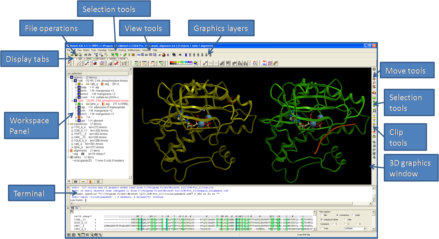
start menu-driven graphical user interface from command line.
The GUI runs the icm.gui file containing all the commands
invoked by menus or pop-ups.
Option simple allows you to keep your terminal window separate from the graphics window.
% icmgl
 gui simple
You can also invoke gui from the command line, e.g.
icm -g # or
icm -g mymenus.gui
icm -G mymenus.gui  # keep the original terminal window
Terminal window and fonts
icm -g (or gui command) invokes a GUI frame with its own built-in terminal window .
To influence the font size in this terminal window, modify XTermFont record of
the icm.cfg configuration file, e.g.
XTermFont *-fixed-medium-*-*-*-24-*
If you prefer to keep the original terminal window use the icm -G option
or invoke the gui simple command from ICM shell (I keep alias guis gui simple
in my personal configuration file). In this case you can change the font of the terminal
window with standard means of the window manager.
3D Graphics window
GUI has a GL-graphics window which can be undisplayed with the
undisplay window
command or from GUI by choosing Clear/No_graphics menu item.
help
Getting help in built-in ICM html browser.
<!--icmscript name="action1"
read pdb "1crn"
display a_*.
-->
...
<a name="action1" href="#action1">click here to execute icm script</a>
help read pdb  # opens the read-pdb section
help "G:learning"
help "I:montecarlo"
help "myfile.html#"
help
help [ input= s_fileName ] [ word1 word2 ... ]
get full help in either text or html form, redirect it to the specified file, if the input
option is specified. Do not use plural forms of the nouns.
Examples:
 help Random
 help read sequence
The built-in help engine does not know about keywords.
It is recommended to use the on-line version of the
ICM manual which has a well-developed Index
(download the newest version of the manual, man.tar.gz from the Molsoft ftp site).
help commands
help commands [ s_Pattern ]
generates concise list of syntax lines for all or specified commands.
help functions
help functions [ s_Pattern ]
generates concise list of syntax lines for all or specified functions.
Examples:
 help                     # type  /stereo, and then letter n or Bar

 help help                # how to get help

 help commands            # list syntax of all commands

 help commands  "rea*"    # list syntax of all read commands

 help functions           # list syntax of all functions

 help functions Matrix    # list syntax of the Matrix family of functions

 help                     # start the browser to use its own search means
 help montecarlo          # just the command name
 help real constant

 help read pdb

 help Split
history
history [ unique | full ] [ i_NumberOfLines]
display previous commands. Option unique squeezes out the
repetitive commands.
Without the full option the commands executed from the file
(rather than manually typed) will not be shown. The unique option
hides the repetitions of the same command.
 history 20              # show last 20 lines
 history unique
To delete all previous history lines, use the delete session
command. In this case the write session command
will save only the new history lines.
if
if
is one of the ICM flow control statements, used to perform
conditional statements.
See also: then, elseif, and endif .
info
Database additional statistics
keep
keep ICM-shell-variable-name1 .. [global]
retain specified ICM_shell variables or their classes (e.g. real, rarray
etc.). This command is used in macros to avoid automatic deletion of
all the local ICM-shell variables.
Also note that four classes
of standard ICM-shell variables,
reals,
integers,
logicals, and
preferences, are automatically restored to their initial
values by default. You can use the keep command to retain their new values.
 macro rdseq s_pdbName  # extract sequence from a pdb-file
   read pdb sequence s_pdbName
   rz = Resolution(s_pdbName,pdb)
   mncalls = 10         # the existing standard shell variable
   keep rz, sequence    # retain all the sequences and rz
   keep mncalls         # retain its new value
 endmacro
s_a = "global"
s_b = "global"
macro m1
  m2
  print "m2: ", "s_a =", s_a, "s_b=" s_b
endmacro

macro m2
  s_a = "m2"
  s_b = "m2"
  keep s_a   # will be kept only for m1
  keep s_b global  # will be kept globally
endmacro

m1
print "global: ", "s_a =", s_a, "s_b=" s_b
join tables
group table t1 {1 2 3} "A"  # 1 has no match in t2
group table t2 {"a" "b" "c"} "A" {2 3 4} "B"
show t1,t2
 #>T t1
 #>-A----------
    1
    2
    3
 #>T t2
 #>-A-----------B----------
    a           2
    b           3
    c           4

join t1.A t2.B name="t3"
t3
 #>-A-----------t2_A-------
    2           a
    3           b
 group table t1 {1 2 3} "A"  # 1 has no match in t2
 group table t2 {"a" "b" "c"} "A" {2 3 4} "B"
 join left t1.A t2.B
 T_join
 #>T T_join
 #>-A-----------t2_A-------
    1           ""
    2           a
    3           b
 group table t1 {1 2 3} "A"  # 1 has no match in t2
 group table t2 {"a" "b" "c"} "A" {2 3 4} "B"
 join t1.A t2.B right name="ttt"
 ttt
 #>T ttt
 #>-A-----------B----------
    a           2
    b           3
    c           4
add column t1 {1 2 3} {1 2 3}
add column t2 { 2 3} {4 5}
join t1.A t2.A local name="t1"
learn from a training data set and create a predictive model
Example:
read table "t.csv"
learn t.A
 learn t.A
 Info> plsRegression model for property 'Apred' built for 95 records.
 Corr_R2=0.44 (CV=0.36),  rmsError=0.48 (CV=0.51)

learn t.pK test=4 select={2,10,20,30} type="pls"
Atom based predictors
Predicting compound properties, using PLS regression or Random Forest classifier/regression on static columns and dynamic chemical `fingerprints.
map={"cd,h;cd,h;cd,h", ";bt;bt", ""} # three chain lengths for atoms, and bonds
Special simplified types for triangle type fingerprints.
number description code comment
9 "atom number" "cd"
3 "hybridization" "sp"
2 "aromaticity" "a"
3 "nHydrogens" "h"
3 "nPolarHydrogens" "hp"
3 "ring/chain" "r"
5 "main valency" "p"
5 "nHeavyNeighbors" "b"
3 "chirality" "c"
7 "sybyl type" "s"
6 "min ring size" "rs"
4 "formal charge" "qfm"
2 "constant" "any"
5 "number of Neighbors" "x"
number description code comment
2 "Donor-Acceptor" "hbda"
2 "Donor" "hbd"
2 "Acceptor" "hba"
4 "aromatic/SP2/aliphatic" "aa"
number description code comment
4 "bond order" "bt"
2 "ring/chain" "r"
2 "rotatable" "rt"
2 "const" "any"
 read table mol "train_set.sdf"
 learn train_set.clogP name="clogPpred" type="plsRegression" \
    test=5 print={1,3,-1,0}  map={"cd,h;cd,h;cd,h", ";bt;bt", ""}
Predict function or predict command can be used to apply the model.
Predict( Chemical("O(C(=O)C)C(C(C(O)=O)=CC1)=CC=1" ) clogPpred )
show Info( clogPpred )
add column clogPpred_w  Info( clogPpred )["fpstat","chains"] name="name"
add column clogPpred_w  Info( clogPpred )["weights"] name="w"
# add column with descriptors for test compounds
add column clogPpred_w Descriptor( Chemical("O(C(=O)C)C(C(C(O)=O)=CC1)=CC=1" ), clogPpred)[1] name="aspirin_desc"
# the value below should correspond to the result of the Predict function for that compound
Sum( clogPpred_w.w * clogPpred_w.aspirin_desc ) + Info( clogPpred )["z"]
Multiple Linear Regression
# add columns with some descriptors
add column Xdict function="MolWeight(mol,'monoiso')" name="MW"
add column Xdict Descriptor(Xdict.mol,number,atom)
M = Matrix( Xdict  {"a_nH", "a_nC", "a_nN", "a_nO", "a_nF", "a_nS", "a_nP", "a_nCl", "a_nBr"} )   # need to make sure all columns have at least one non-zero value
calcMLR M Xdict.MW

W = R_out    # weights

#To apply weights back

 add column Xdict name="molW_pred"  M * Transpose( Matrix(W ) )[?,1]
Corr( Xdict.MW Xdict.molW_pred )
Building deep learning ANN models with ICM for Predicting compound properties
Building descriptor based ANN model
Example:
print = Collection( 'ATMAP' 'cd,h', 'BOMAP' 'bt', 'TYPE' 'ecfp', 'SIZE' -1, 'BINARY' yes, 'ECFPITER',3 ) # ECFP4 fingerprint
Example:
Collection( "op" "fc" "num_hidden" 5, "act", "sigmoid" ) # FullyConnected layer with 5 hidden neurons and sigmoid activation
Example:
net["optimizer"] = Collection( "learning_rate", 0.005, "stochasticGrad", yes )
Example (model to predict LogP values)
net = Collection()   # empty collection to define network
layers = Array()     # array with network layers
# two layers
layers[Nof(layers)+1] = Collection( "op" "fc" "num_hidden" 5, "act", "sigmoid" )
layers[Nof(layers)+1] = Collection( "op" "fc" )
net["layers"] = layers
net["optimizer"] = Collection( "learning_rate", 0.005 ) # optimizer parameters
# final learn command to build a model to predict 'logP' column for table t using counted ECFP4 as descriptors
learn number=50 test=t t.logP name="logPpred" type="nnetreg" network=net \
                print = Collection('ATMAP' 'cd,h', 'BOMAP' 'bt', 'TYPE' 'ecfp', 'SIZE' -1, 'BINARY' no, 'LEN' 100, 'MINLEN' 1 'ECFPITER',3 )
Building convolutional ANN model
description code
simple organic map "cd"
Mendeleev map(6-bits) "cdm"
nHydrogens "h"
formal charge "qfm"
nRings "r"
hybridization "sp"
HBD "hbd"
HBA "hba"
nHeavyNeighbors "b"
ExtraColumns "ex"
sp1 hyb "sp1"
sp2 hyb "sp2"
sp3 hyb "sp3"
nNeighbors "x"
MinRing3 "r3"
MinRing4 "r4"
MinRing5 "r5"
MinRing6 "r6"
Example (model to predict LogP values using chemical convolutional network)
net = Collection()   # empty collection to define network
layers = Array()     # array with network layers
# two chemical convolutional layers with activation
layers[Nof(layers)+1] = Collection( "op" "conv", "type", "chem", "num_filter" 20, "act", "sigmoid")
layers[Nof(layers)+1] = Collection( "op" "conv", "type", "chem", "num_filter" 20, "act", "sigmoid")
# pooling summation layer
layers[Nof(layers)+1] = Collection( "op" "pool", "type", "sum" )
# fully connected layer (set num_hidden to number of properties per-compound you're training on)
layers[Nof(layers)+1] = Collection( "op" "fc"  "num_hidden" 1 )
net["optimizer"] = Collection( "learning_rate", 0.005 ) # optimizer parameters
# final learn command to build a model to predict 'logP' column for table t
# using single atom properties and chemical graph
learn number=500 test=t t.logP name="logPpred" type="nnetreg" network=net chemical='cdm,h'
Full list of supported layer/operator types
Link the graphical object to one or several molecules, or an object move in 3D space together
read pdb "1xbb"
cool
make grob skin a_asti a_asti # grob g_1xbb_asti is created
make grob skin a_a a_a # grob g_1xbb_a is created
color g_1xbb_asti yellow
display grob
link g_1xbb_asti a_asti
Field( a_asti "_GROBLINK_" )
#  {g_1xbb_asti}
connect a_asti # move it and grob will move with it. Then press Esc to disconnect
#
link g_1xbb_a a_A
Field( a_A "_GROBLINK_" )
#  {g_1xbb_a}
Link or assign reaction group arrays to a Rx positions on a chemical scaffold.
extract the R-group associated with the given position from the scaffold
into a stand-alone shell
chemical table.
One can read an RG file with a scaffold and RGroups and a scaffold with linked,
but hidden, arrays will be created. Then these arrays can be turned into external
chemical tables, edited and linked back to the scaffold.
write table mol scaffold "markush.mol" # creates an RG file
#
read table mol "markush.mol"
enumerate library scaffold.mol
link internal variables of molecular object
link vs_varChainToBeLinked
impose a chain of equality constraints
(v[1] = v[2] = v[3] = ... = v[n])
on the specified variables
(or, in other words, keep the specified variables equal to each other).
If one of the variables is changed all the others will be changed.
Energy derivatives are modified accordingly.
This command is great for modeling periodic structures
(e.g. (Pro-Glu)n).
# single chain
build string "ala ala ala ala ala ala ala ala ala ala" # 10 alanines
link v_//phi # all the phi angles should be equal
link v_//psi # all the psi angles should be equal
montecarlo v_/2/phi,PSI v_* # sample just one residue
# multiple chains for a dimer
delete a_*.
build string "leu ala ala leu ala ala ala leu"
copy a_ "b"
mv a_2. a_1.
ds a_
set v_1//tvt1 0.
set v_2//fvt1 180.
fix v_//tvt1,fvt1 # do not link those
link v_//* molecule
montecarlo v_1/* v_/*
Be careful with selections of psi variables in peptides since they
are assigned in ICM to the first atom of the next residue. PSI
specification goes around that attribution.
delete link variable
command.
Link chains/molecules to sequences and alignments
link ms [ali1 .. [only] | alignment | sequence | seq1 seq2 ... seqN]
link or associate protein molecules with separate sequences or sequences
grouped in an alignment. If alignment ali_ is given, molecules
are also linked to this alignment (note that the same sequence can be
involved in several different alignments).
Amino-acid sequences of amino- or nucleotide- chains in molecular selection
ms_ will be compared with specified ICM-shell sequences
and identical pairs will be linked. Make sure that you specify one
molecule selection, use logical or (|) between the two selections if
necessary. Linking molecules with alignments allows an automatic
residue-residue assignment by the following commands and functions:
superimpose, set tether, Rmsd and Srmsd .
Alignments can be prepared in advance either automatically by the
align command or Align
function, and/or modified by manual editing of the alignment file.
The following illustrates the first step of homology modeling.
Example:
build "newseq" # that is what you want to build by homology
read pdb "template.pdb" # that is the known pdb-template
read alignment "seq3Dali.ali" # prepared/modified sequence alignment
# of the two structures
set object a_1. # this is the first molecule that we
# are going to model
link a_*. seq3Dali # establish links between sequences
# and objects
set tether a_1,2.1 seq3Dali # impose tethers according to the alignment
minimize tether # fold it according to the template
list
list ICM-shell objects matching the name pattern (all if name-pattern
is omitted). The plural form can be used for more natural expressions.
'list commands' actually means list all legal words known by ICM (ICM
command words). Use flanking asterisks to search in any position.
Option find or pattern automaticall transforms unquoted word into "*word*"
Examples:
list # list the "most wanted" object-types
list functions
list sequences # if you have aliases, you can
# type 'ls se' instead
list "*my*" # all ICM-shell variables containing "my"
list find my # the same as the previous search
list pattern my # identical to the previous too
list graphic font : listing existing fonts for 2D and 3D graphics labels
list graphic font
-#-F-sz-biu-rf
1 2 24 1
list the content of the icm binary file
list binary [ s_binaryFileName ]
list the table of contents of the icm-binary multi-object file.
The default name is -"icm.icb" and the default extension is ".icb" .
To read the whole archive, use the read binary command.
For a subset of objects, add the name= S_listOfNames option.
Note that the archive can also store graphical view parameters,
tethers between the objects, and a string buffer with the last
session.
Example:
list binary s_icmhome + "example_docking"
Binary file version: 1
1 mn_saveAll integer 4
2 a integer 4
3
read binary list s_icbfilename name= s_TOC_table_name read binary s_file name= S_objects_of_interest
list available sequence databases
list database
gives a list of BLAST databases which can be used by the find database command for fast
sequence database searches.
Normally, your system administrator should update the BLAST sequence files. ICM just needs a path
to this directory which is defined by the $BLASTDB system variable.
The output of the command is saved in the S_out array.
This array can further be processed with the Field function.
Example:
list database
dblist = Field(S_out, 2) # sarray contains search databases
show dblist
a=Sequence("PDPPLELAVEVKQPEDRKPYLWIKWSP")
find database a dblist[2]
Trouble-shooting: If you get an error message, check the following:
list directory
list molcart
load
load conformation from stack
load conf i_confNumber [ sstructure ]
assign the i_confNumber-th conformation from the shared conformational stack (not to be confused with the embedded object stack)
and to the current object (e.g. when you browse conformations accumulated after a montecarlo run).
If i_confNumber is zero, the best energy conformation will be loaded.
Montecarlo stack conformations are sorted according to energy values,
however you may create your stack manually with an arbitrary order.
Option sstructure will automatically recalculate the secondary structure according to the hydrogen bonding pattens.
Note that the full energy of this conformation
which had been stored in the stack can be accessed by the Energy("func") function.
If an object os1 is specified, the conformation is loaded from the object-embedded stack stored in the specified object. If the second object is specified the conformation will be transferred to the target object.
The command will update the information about the current conformation in the object's stack.
read stack "f1" # read conformational stack
load conf 0 # set molecule into the best energy conformation
display a_//ca,c,n # display the backbone
for i=1,Nof(conf) # go through all the conformations
load conf i # load them one by one
print Energy("func") # extract its energy
pause # wait for RETURN
endfor
#
store stack a_ # move stack to an object
delete stack # delete shared stack but keep the in-object one.
load conf a_ 1
load trajectory frame conformation
load frame i_trjFrameNumber [ s_trjFileName ] [ sstructure ]
load specified frame from the trajectory.
Note that the full energy of this conformation
which had been stored by the simulation procedure
can be accessed by the Energy("func") function.
Option sstructure will automatically recalculate the secondary structure according to the hydrogen bonding pattens.
Examples:
build "alpha" # build extended chain of the Baldwin peptide
read trajectory "alpha"
display trajectory "alpha" center # a-ha! conf in frame 541 is interesting
load frame 541 "f1" # extract conformation from frame 541
print Energy("func") # print its energy without recalculating
create database table view
load a structural alignment solution
load solution [ i_solutionNumber ]
loads the specified solution previously stored by the
align rs_residue1 rs_residue2 .. command.
The two output selections as_out and as2_out contain equivalent residues of the
specified solution. The second object will be superimposed according to the Ca atoms of the
found equivalent residues.
Example:
read pdb "4fxc"
read pdb "1ubq"
display a_*.//ca,c,n
color molecule a_*.
align a_1.1 a_2.1 12 1.5 .1
center
load solution 2 # load the second best solution
color red as_out
color blue as2_out
for i=1,10
load solution i
color molecule a_*.
color red as_out
color blue as2_out
pause # rotate and hit 'return'
endfor
load conformational stack from an object
read object "objeWithStack.ob"
if(Exist(a_ stack)) load stack a_
load object from parray or parray in a collection
load object objArr [name=s] [delete]
read pdb "1crn"
read pdb "2cpk"
p = Parray(object)
delete a_.
load object p[2]
#
c = Collection()
c["ob"]=a_1.
delete a_*.
load object c["ob"] name="x"
load object c["ob"] name="x" delete # overwrite the previous a_x.
ICM-shell macros and functions
a named group of ICM commands with arguments that can be called and executed from the ICM shell.
A very similar entity is a user-defined (or icm-shell) function that is like a macro but may return a value and be nested.
Macros of functions can be :
Macro can call another macro (nested macros).
Syntax of the macro definition:
macro macroName [mute|auto] prefix1_macroArg1 [(default1)] prefix2_macroArg2 [(default2)] ...
macro creates_a
# commands
a=1
keep a # used to push 'a' to the upper level, 'keep global' for all levels.
endmacro
creates_a # calling macro a
show a # checking if it creates variable 'a'
Example of a simple macro with arguments:
macro countMetalNeighbors as_ r_dist (5.)
l_commands = l_info = no
nMetals = Nof( Mol( Sphere( as_ , a_*.M , r_dist ) ))
print " nMetals = ", nMetals
keep nMetals
endmacro
read pdb "1are"
countMetalNeighbors a_/his,as* 4.
function Bold( s ); return "<b>"+s+"</b>"; endfunction
Bold("Hey") # returns "<b>Hey</b>"
See also function .
Defaults can be provided in parentheses as simple constants (i.e.
i_window (8) ), or as the whole expressions
(i.e. i_1 (mncalls) r_a (Sin(*2.)) i_2 ) . Default expressions can also be omitted.
Options
The predefined standard ICM-shell
integer,
real,
and
logical
variables, as well as
preferences
(i.e. i_out, l_warn, wireStyle, PLOT.logo etc.)
are be automatically restored upon completion, if changed in the macro, to
retain the new value use the
keep
command. Note that the string variables should be restored explicitly.
Many
macros
are supplied with the program.
Examples:
# display molecule as a worm colored from N- to C- term.
macro dsWorm ms_ (a_*) r_wormRadius (0.9)
GRAPHICS.ribbonWorm = yes
GRAPHICS.wormRadius= r_wormRadius
display ms_ ribbon only
for i=1,Nof(ms_) # color each molecule separately
color Res(ms_[i]) Count(Nof(Res(ms_[i]))) ribbon
endfor
endmacro
To invoke the macro, type
read object s_icmhome+"crn"
dsWorm a_1 0.7
or just
dsWorm # and press Enter
A set of ICM macros is given in the _macro file.
make
make background : spawning background jobs and processing their output.
make background "ls > tmp.txt" command="read string \"tmp.txt\" " info=""
# the empty info arg suppressed the dialog
show s_out
#
make background name="job1" Path(unix,"_myScript",{"-n","-s"})
# Path(unix,..) returns current ICM location
A Windows example:
make background "\"c:\\Program Files\\Microsoft Office\\WINWORD.EXE\" C:\\Temp\\Doc1.doc" simple
make bond: forming a covalent bond
make bond as_singleAtom1 as_singleAtom2 [type=i_type]
The type= option allows one to set the bond type ( i_type ={1|2|3|4} ,
for a single (default), double, triple and aromatic bond, respectively.
build string "ala ala ala ala ala"
make bond simple a_/1/n a_/5/c
set term "bb,bs,af"
minimize
make bonds in an atomic chain
make bond chain as_chainOfAtoms
connects specified atoms in a linear chain. Useful for PDB entries
containing only Ca atoms.
Examples:
read pdb "4cro" # contains only Ps and Ca's
display # Milky sausage
make bond chain a_4cro.//p # connect P atoms of the DNA backbone
make bond chain a_4cro.//ca # connect Ca atoms of the protein backbone
See also:
delete bond.
make boundary: Poisson electrostatics
a command to prepare for the boundary element electrostatic calculation
make boundary [as]
this is an auxiliary command which is required if you need to calculate the
electrostatic free energy with the boundary element method several times.
Optional atom selection as_ from which the electrostatic field is calculated
can be specified.
This may be the case if the charge distribution changes but the shape does not.
However, the boundary does depend on the dielectric constant parameters such as
dielConst and dielConstExtern . If you intend to change them the boundary need to
be remade every time.
This command does not generate any output by itself,
it just creates the internal table which can later be used by the
show energy command or the Potential( ) function.
The dielectric boundary is a smooth analytical surface which is built with the contour-buildup
algorithm ( Totrov,Abagyan, 1996 ). The surface looks like the skin surface, but uses
different radii which were optimized against experimental LogP data. Both skin and the dielectric
boundary uses the same water radius ( the waterRadius parameter). The "electrostatic"
radii used by ICM to calculate the boundary are stored in the icm.vwt file.
See also:
REBEL,
surfaceAccuracy,
electroMethod,
delete boundary,
show energy",
term "el",
Potential( ).
Examples:
electroMethod="boundary element"
read object s_icmhome+"rinsr"
delete a_w* # get rid of water molecules
make boundary a_1 surfaceAccuracy = 5 # calculate params of the dielectric boundary
show energy "el" # electrostatic energy by BEM
e1=Energy("el") # extract the energy
set charge a_/33/cd*,hd*,ne*,he*,cz,nh*,hh* 0. # uncharge arg33
show energy "el" # electrostatic energy of the uncharged Arg33
e2=Energy("el") # extract the energy
print e1-e2
delete boundary # memory cleanup
make directory
make specified directory. Example:
make directory "/home/doe/temp/"
See also: sys , set directory, delete directory, Path(directory)
make disulfide bond
make disulfide bond [ only ] as_atomSg1 as_atomSg2
form breakable disulfide bonds between two sets of specified sulfur Sg atoms,
regardless of the distance between them. Forming the bond means that two
Hg hydrogens of Cys residues are dismissed, a covalent bond between two Sg
is declared (but not enforced)
and four local distance restraints (see
icm.cnt)
are imposed. These restraints are indeed local, since two Sg atoms only start
feeling each other when they are really close, otherwise the energy contribution
is close to zero
. Option only causes deletion of previously formed
disulfide bonds, otherwise the new one is added to the existing list of
disulfide bonds.
build string "se cys ala cys" # sequence containing two cysteins
display # display an extended ICM model of the sequence
# set only one SS-bond, disregard all previous
make disulfide bond a_/1 a_/3 only
montecarlo # MC search for plausible conformations
See also:
delete disulfide bond
and (important!)
disulfide bond.
make drestraint: extract distances structure
make drestraint as_select1 as_select2 r_LowerBound r_UpperBound r_LowerCorrection r_UpperCorrection [s_fileNameRoot]
create two files containing the list of all the atom pairs specified by
two selections (i.e. a_* a_* - all the pairs; a_1//* a_2//* atom pairs
between molecules 1 and 2 for which the interatomic distance lies between
r_LowerBound and r_UpperBound.
Note: it is critical that both selections are in the same object.
Only tethers can pull to atoms of a different object.
For each pair of atoms a
distance restraint type
is created with lower bound less than the actual interatomic distance by
r_LowerCorrection and upper bound greater than the actual
interatomic distance by r_UpperCorrection. This command can be
used for example to impose loose distance constraints between two subunits.
The number of the formed drestraints is returned in the
i_out variable.
See also:
set drestraint as_1 as_2 i_Type
if you want to impose a specific drestraint.
Examples:
read object s_icmhome+"complex" # load a two molecule complex for refinement
# extract all Ca-Ca pairs between 2 and 5 A
# for each pair at distance D create distance
# restraint type with lower bound D-2.5 and
# upper bound D+2.5
make drestraint a_1//ca a_2//ca 2. 5. 2.5 2.5
make factor: FFT calculation of diffraction amplitudes and phases
make factor map_Source {I_3Maximal_hkl | r_resolution} [s_factorTableName[s_ReName[s_ImName]]]
calculate structure amplitudes and phases from the given electron density
map by the Fast Fourier transformation. The table ' s_factorTableName'
with h,k,l and structure factors
will be created (further referred to as T for brevity).
It will contain the following members:
If structure factor table s_factorTableName already exists,
structure factor real and imaginary components are created or updated
in place. Any other arrays containing experimental, derivative or control
information may be added to the table and participate in selections and sorting.
Example:
read map s_icmhome+"crn" # load "crn.map"
set symmetry m_crn 1
make factor { 5 5 5 } "F" # h_max=k_max=l_max=5
# F.h, F.k, F.l, F.ac, F.bc are created
show F
group table append F Sqrt(F.ac*F.ac + F.bc*F.bc) "Fc" Atan2(F.bc,F.ac) "Ph"
sort F.Fc
show F
make flat chem_array
read table mol s_icmhome+"template_3D.sdf"
make flat template_3D.mol
See also: Chemical , read table mol .
make grob map command to contour electron density or grid potentials
make grob m_map [header] [solid] [box] [I_indexBox[1:6]] [[exact] [field=]r_sigma|r_absValue] [as [margin=r]] [name=s]
Example:
build string "his glu"
make map potential Box( a_ 3.)
make grob m_atoms 3. # 3 sigmas above the mean
# make grob m_atoms .2 exact # countour at 0.2 level
# .2 or .1 exact is useful to detect almost closed pockets
display g_atoms
#
make grob m_atoms exact 0.15 # at value of 0.15
display g_atoms
#
mapSigmaLevel = 1.5
make grob m_atoms add 0. # at mapSigmaLevel
make grob g_atoms add -0.1 # at 1.4 sigma
#
loadEDS "1atp" 0.
read pdb "1atp"
make grob m_1atp 1.5 a_atp
cool a_
display g_1atp
Defaults:
Option solid tells the program to create a solid
triangulated surface which can later be displayed by
display grob solid
command. The threshold is expressed in the units of standard deviations
from the mean map value, i.e. 1.0 stands for one sigma over the mean.
I_indexBox [1:6] is optional 6-dimensional
iarray
containing
{ i_startSection i_startRow i_startColumn i_NofSections i_NofRows i_NofColumns }.
It overrides the default, contouring the whole map.
Option box adds surrounding box to the grob.
make grob image command to create a vectorized graphics object.
make grob image [name=s_grobName]
create a vectorized
graphics object (grob)
from the displayed wire or solid objects. The information about colors will be
inherited. Very useful if you want to export wire,
ribbon
or CPK into another graphics program, since graphics objects can be
written
in portable Wavefront (.off) format. Further, graphics objects can exist
independently on the molecules which may be sometimes convenient. Also, underlying
lines and vertices can be revealed. The graphics object created from the displayed
solid representations assigns and retains color information as lit in a given
projection. These colors can not be changed. Use special
make grob skin
command to generate a more elaborate graphics object from skin .
Examples:
read object s_icmhome+"crn"
ds a_crn.//!h* ribbon # ribbon
make grob image name="g_rib"
display g_rib smooth only # try select g_rib and Ctrl-X,Ctrl-E/W etc.
# option smooth eliminates the jaggies.
write g_rib # save to a file
make grob matrix
make grob [solid] [bar[box]] [color] M_matrixName [r_istep r_jstep r_kstep] [[name=]s_grobName]
 Create a three-dimensional plot from M_matrixName, so that
x=i* r_istep, y=j* r_jstep and F(x,y)= k* M_matrixName[i,j].
Options:
Create a three-dimensional plot from M_matrixName, so that
x=i* r_istep, y=j* r_jstep and F(x,y)= k* M_matrixName[i,j].
Options:
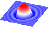
Examples:
read matrix s_icmhome+"def"
make grob def solid
display
# OR
read matrix s_icmhome+"ram" # phi-psi energy surface
make grob ram 1. 1. 0.1 # create the surface
display g_ram magenta # display it
make grob solid ram 1. 1. 0.08 name="g" # create the surface
display g solid gold # display it
make grob potential
make grob potential [solid] [as_1 [as_2]] [[field=]r_potentialLevel] [grid=r_gridCellSize] [margin=r_margin] [[name=]s_contourGrobName]
make grob potential a_lig
create graphics object of isopotential contours of electrostatic potential
which takes not only the point charges but also the dielectric surface charges
resulting from polarization of the solvent.
This potential need to be calculated in advance by the
boundary element algorithm.
Contours can be displayed in the wire and solid representations (see also
display grob). The default parameters are:
See also:
make map potential,
electroMethod,
make boundary,
show energy "el",
term "el",
Potential( ).
Examples:
build string "se his arg glu"
electroMethod="boundary element" # REBEL algorithm
make boundary
make grob potential solid 0.1 grid=2. margin=4. name="g_equipot1"
display g_equipot1 transparent blue
make grob potential solid field=-0.1 grid=2. margin=4. name="g_equipot2"
display g_equipot2 transparent red
ds xstick residue label
make grob skin or surface
make grob skin [wire | smooth] [as_1 [as_2]] [[name=]s_grobName] [r_transparency]
create grob containing the specified molecular surface (referred to as skin).
If the wire option is given the transparent wire grob
will be created (solid grob is the default).
It will have the same default color.
The disconnected parts of this grob may later be split .
The grob will be named by the default name g_objName unless
the name is explicitly specified.
The final actual name will be returned in s_out .
The smooth option allows one to close the cusps. This closure is necessary to
enable the compress grob operation.
The compress g_ command allows one to dramatically simplify the triangulated surface
and reduce the number of triangles. Typically compress g_ 1. will reduce the
number of triangles by an order of magnitude.
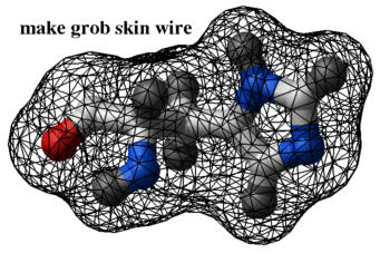
A grob can later be colored with the color grob potential command.
Examples:
read object s_icmhome+"crn"
# skin around a substructure, (just as an example)
make grob skin a_/1:44 a_/1:44 0.6
split g_crn_m
display g_crn_m2 a_//*
show Area(g_crn_m2), Abs(Volume(g_crn_m2))
make grob skin a_ a_ name="gg1" # display gg1 now
make grob skin wire name="gg2" # display gg2 now
make grob skin smooth a_/1:20 a_/1:20 name="gg3"
compress gg3 1. # simplifies the surface
The transparency can also be set with the set grobname r_transparencyLevel
command.
Creating 3D label objects
name = s_n the name of the created array of 3D labels
append append new 3D labels to the existing array;
delete forcefully delete the array before repopulating it with 3D labels;
refresh keep all existing 3D labels which are outside the specified selection, rebuild 3D labels inside the selection;
display display the created labels.
make distance
make distance as_1 [as_2|auto] [molecule|align] [r_maxdist] [3d label options]
read object s_icmhome+"crn"
display ribbon wire
make distance a_//oe* a_//ne,nh* display
make distance a_//oe* a_//ne,nh* 5. delete display
make distance a_//!vt* a_//!vt* 1.5 # creates a distance object
CLASHES = Table( $s_out distance ) # s_out stores name of distance-object
sort CLASHES.dist
show CLASHES.dist<0.8
make hbond
make hbond as_1 [as_2 | auto] [molecule | align] [r_maxdist] [3d label options]
Examples:
read object s_icmhome+"crn"
display ribbon wire
make hbond a_ display GRAPHICS.hbondMinStrengh=0.5 name="x"
t = Table(x,distance)
sort t.dist
show t[1]
make angle
make angle as_3_connecting_atoms [3d label options]
make torsion
make torsion as_4_connecting_atoms [3d label options]
read object s_icmhome+"crn"
display ribbon wire
make angle a_/22/c | a_/23/n,ca display
make torsion a_/22/ca,c | a_/23/n,ca display
make/store graphical image to image parray
make image # will create album if it does not exist
make image #
make image #
delete variable album 2
make key # obsolete
make key {s_smiles | as} [S_arrayOfFragmentSmiles]
Note: the make key command is obsolete. The new chemical fingerprints are dynamic and
does not have a predefined set of fingerprints of variable length.
The new fingerprints are used in the following commands and functions:
By default the make key command uses a built-in array of 96 substructures,
and generates a 24-character hex-string ( each hex-character codes for 4 bits ),
however any string array of subfragment smile-strings ( S_arrayOfFragmentSmiles )
can be provided.
The hex-string can be converted back into an array of bits packed into
integers with the Iarray( { s_chemkey | S_chemkey } key ) function.
The bit-distance matrix between two arrays of bit-strings represented by two iarrays
can be calculated with the
Distance( Iarray( S_1 key ) Iarray( S_2 key ) i_nBits [ key ] ) or
Distance( Iarray( S_1 key ) Iarray( S_2 key ) i_nBits simple )
functions, where the number of bits, i_nBits, is usually 96,
unless you use a user defined array of fragments. There is also a weighted form
of the chemical key distance (see the Distance function).
By default, or with the key option, the function returns matrix with
the Tanimoto similarity distance (0. all bits are the same, 1. no bits in common),
while with the simple option the second chemical key is considered as
a sub-fragment and the distance becomes 0. (identity) if the sub-fragment is
present in the first bit-mask.
Examples:
read mol s_icmhome+"ex_mol.mol"
S_key = Sarray()
for i = 1, Nof(a_*.)
set obj a_$i.
build hydrogen
set type mmff
convert
smil = Smiles(a_)
make key smil
S_key = S_key // s_out
delete a_
endfor
S_key
make map
make map cell
make map cell R_6cellParameters I_3NofSteps [R_6box | I_6box] ["zxy"] [as] [name=s_mapName]
create an electron density distribution for atom selection as_
(all atoms of the current object by default) on a three-dimensional grid.
See also make map potential for a rough electron density map.
The electron density is calculated from the cartesian coordinates of the
selected atoms using a 2-Gaussian approximation. If the l_xrUseHydrogen logical
is set to no , hydrogen atoms are ignored.
The following parameters are taken into account:
R_6cellParameters is a real array containing { a b c alpha beta gamma } parameters. Optional
R_6box or I_6box arrays define the corner of the map box
(closest to the origin) and its sizes
( { x1 y1 z1 dx dy dz } or { nx ny nz dnx dny dnz }, respectively).
The whole cell is taken by default.
Examples:
read object s_icmhome+"crn"
make map cell {5. 5. 5. 90. 90. 90.} 0.5 a_//ca,c,n
make map factor : calculate electron density map from structure factors
make map factor [T_factor] [m_map]
calculate an electron density distribution on a three-dimensional grid from a
structure factor table of the Miller indices, reflection amplitudes and phases.
Requires that the map is created before with the make map command.
If optional arguments are not given the current map
and/or current factor will be used.
A new empty map can be created from an empty selection by the
make map a_!*
parameters # see the
make map cell command.
make map potential: grid energies, converting crystallographic electron density maps
create a property map for the as_ selection.
This command is used for low-resolution surface generation or to make
grid potential maps for fast docking.
The optional arguments are the following:
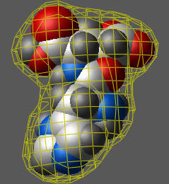
m_atoms contoured at 0.3 exact level. The 0.5 level is closer to the van der Waals surface.
build string "his arg"
display cpk
make map potential Box( a_ 3.)
# wire surface
make grob m_atoms 0.3 exact # contours near vw-radius.
display g_atoms
# solid surface
make grob m_atoms solid 0.5 exact
display g_atoms smooth
build string "se his arg"
make map potential "el" Box( a_/1,2/* , 3. )
display a_
display map m_el {1 2 3}
make grob m_el exact # contouring at 0. potential
display g_el
set occupancy a_/arg/!ca,c,n,o,cb 0.3
make map potential simple occupancy "gc" Box( a_/1,2/* , 3. )
# enforce a single map with attenuated side chain
Fine-tuning the maps
Sometimes you want the van der Waals grids, "gh" and "gc", generated from the whole receptor,
while the "ge" or "gb" grids generated only from a small region of the receptor.
In this case you can run the command two times with different source-atom selection.
Example:
read object s_icmhome+"crn"
make map potential "gh,gc" a_1 Box(a_1)
make map potential "gb,ge,gs" a_1/15:18,33:46 Box(a_1)
write m_ge m_gc m_ge # write three maps at once
A different method is to use the
Bracket( m, R_6box ) function which sets
everything beyond the box to zero. Noted that the in the above method only the selected residues make contribution.
In the following method all residues make contribution, and then the resultant map is truncated in space. Example:
rename m_ge m_ge1 # Compare with the map generated in previous example
make map potential "gh,gc,gb,ge,gs" a_1 Box(a_1)
m_ge = Bracket(m_ge, Box( a_1/15:18,33:46 )) # redefine m_ge
display m_ge
display m_ge1
make molcart
add column t Chemical({"CCC","CCO"}) # create a local table
make molcart table t name="test.t" # copy it to molcart
make molcart table input="test.t" name="test.tt" # make another copy
make molcart table input="test.t" name="test.tt" append # append the same table again
print Nof( "test.t" sql ), Nof( "test.tt" sql ) Nof( "test.tt" molcart unique )
SAR analysis
group table t Chemical( { "C1NC(C(C1O)O)CO","C1NC(C(C1O)C)CO" } )
make molsar t Chemical("C(NCC1)C1") auto name="tsar1"
make molsar t Chemical("C(NC(C1)[R1])C1[R2]") auto name="tsar2"
split molsar: generate SAR table from the result of `make-molsar
group table t Chemical( { "C1NC(C(C1O)O)CO","C1NC(C(C1O)C)CO" } )
make molsar t Chemical("C(NC(C1)[R1])C1[R2]") auto name="tsar2" append
split molsar tsar2.R1 tsar2.R2
make pca
make peptide bond
make peptide bond as_C as_N_or_S
form the peptide bond between two selected C- and N- atoms, or the thioester bond
between C- and S- atoms. The bonds may be formed
between the terminal amino- and carboxy- groups (a_/1/n and the last c),
as well as between such amino acid side-chains groups as
a_/lys/nz and a_/asp,asn/cd, a_/glu,gln/cg.
The energy restraints for form the additional chemical bond will be calculated under the "ss" term
and can be viewed with show drestraint
See also:
delete peptide bond
How to modify an ICM-object .
Example:
build string "se nh3+ gly gly gly gly gly his" # notice: NO C-term group
display
make peptide bond a_/nh3*/n a_/his/c # form a cyclic peptide
# display drestraint
minimize "ss"
minimize "vw,14,hb,el,to,ss"
#
# form thioester bond
#
build string "se cys ala ala ala glu"
display
make peptide bond a_/1/sg a_/5/cd
minimize "ss" # term "ss" is responsible for the extra drestraints
make bond simple .. ..
set term "bb,bs,af"
will use the force field to keep the peptide closed.
Generate an attractive grid map from crystallographic electron density map for refinement
loadEDS "1atp" 0. # downloads electron density map m_1atp
read pdb "1atp"
make map potential m_1atp a_atp # map around around ATP
m_gc = - m_xr # a possible use. Also possible with "gp"
set terms "gc" # add gc germ for minimization
make plot: Adding a scatter plot or a histogram to a table
x="Random(1.,10.,100)"
add column t $x $x Shuffle(Sarray(50,"red")//Sarray(50,"blue")) $x $x name={"x","y","C","S","sz"}
make plot t "x=A;y=B;color=C;shape=D;size=E;" # or
make plot t "x=A;y=B;color=C;;element=rectangle;center=1.3,2.4;radii=1.3,2.0;color=red"
add header t Matrix(10) name="mt"
make plot t "matrix=mt;rainbow=white/yellow/green"
Scatter plot arguments
group table t Random(1. 10. 40) Random(1. 10. 40) Iarray(20,0)//Iarray(10,1)//Iarray(10,2)
make plot t "x={A,B}"
make plot t "x=A:C"
group table t {300. 200. 500.} "Volume" {390. 230. 630.} "Area" {5 3 1} "i"
x = "x=Volume;y=Area;color=i;size=8;;title=Volumes and areas;;"
y = "element=rectangle;x1=150;y1=200;x2=550;y2=550;color=blue;fillStyle=BDiagPattern;label=Drugs;labelPos=center"
make plot t x+y
add column t Random(100,0.,1.) Random(100,0.,1.) Random(100,0.,1.)
make plot t "x=A;y=B;color=C;size=6;style=dots;;" output="aaa.png" size = {500,500}
unix display aaa.png # display the plot using Linux 'display' program
General properties are also applicable after two semi-colons: ( xTitle , yTitle , title )
Example:
read pdb "1crn"
m = Matrix(a_/A a_/A ) # residue contact matrix
add header t m name='m'
make plot t "matrix=m;rainbow=white/yellow/green;depth=-1;legend=m;;xTitle=I;yTitle=J;title=Contacts of Crambin"
make reaction : applying reaction to the products
Parray("[R1]C(=O)O.N[R2]>>[R1]C(=O)N[R2]" )
Note that here the dot . separates the reactants and the >>
indicate the reaction.
Example:
m1 = Parray( { "C(C(=O)O)(=C(C=C1)N)C=C1SC#N" "C(=CC(=C(O)C1)C=CC=1)(C(=S)N)C(=O)O"\
"N(=C(S1)N)C(C1=CC(C=C1)=CC=C1C(=O)O)=O" "C(C(=O)O)(C(=CC1)N)=CC=1N=C=S" } )
m2 = Parray( { "C(C(=O)O)(=C(C=C1)N)C=C1SC#N" "C(=CC(=C(O)C1)C=CC=1)(C(=S)N)C(=O)O"\
"N(=C(S1)N)C(C1=CC(C=C1)=CC=C1C(=O)O)=O" "C(C(=O)O)(C(=CC1)N)=CC=1N=C=S" } )
make reaction Parray("[R1]C(=O)O.N[R2]>>[R1]C(=O)N[R2]" ) m1 m2
make reaction Parray("[R1]C(=O)O.N[R2]>>[R1]C(=O)N[R2]") m1 m2 filter="MolWeight(mol)<400 & MolLogP<6"
react = Parray("[R1]C(C(=O)[R2])=O>>C1C(=C(C=CC=1)[R2])[R1]")
rct1 = Chemical( {"CC(C(C)=O)=O", "CC(C(c1ccccc1)=O)=O"} )
make reaction react rct1 filter = "R1==R2"
make reaction react rct1 filter = "R1!=R2"
read binary s_icmhome + "example_reaction1.icb"
make reaction r_han_pyr.rxn[1] name=Name( "T_react", unique ) reactant1.mol,reactant2.mol
filter = "MolLogP<5. & Nof_Frags('C(O)=O')<1"
make sequences from alignment
take a vertical block from an alignment and convert it into a separate
alignment with independent truncated sequences.
read alignment s_icmhome+"sh3"
make sequence sh3[20:50]
See also:
make sequence: extract from pdb or icm structure
creates sequences (or, more strictly speaking, ICM-shell objects of the 'sequence' type)
of residues composing selected molecules ms_ .
One-letter equivalents of full residue names are specified in the icm.res library.
Option resolution adds the X-ray resolution value multiplied by 10 to the name
(e.g. 2ins_a25 for resolution of 2.5A) or 'No' for NMR and theoretical structures.
The group sequence command will automatically prefer a sequence from
structure with better resolution.
The resolution is not appended if option name= is specified.
The make sequence command also extracts both the secondary structure
and the site information.
See also: read pdb sequence
Examples:
read pdb "2ins"
make sequence a_2ins.a,b # two seqs 2ins_a and 2ins_b created
make sequence a_2ins.a,b resolution # resolution*10 added to the name
make sequence a_1.1 name="aa" # sequence named: aa
make sequence a_2ins.a,b name={"aa","bb"} # seqs named: aa and bb
make random sequences
make sequence 10 # makes sq1,sq2,..
make sequence 10 name='seq' # seq1,seq2
make sequence 10 40 # 10 sequences with len=40aa
make sequence 10 40 50 # 10 sequences with len=40 to 50aa
make tree
read table "t.tab" name="t"
make tree t
read table "t.tab" name="t" # N rows
make tree t full # all distances between rows are calculated
# or
read matrix "dist.mat" name="dm" # N x N matrix
group table t append header dm
make tree t distance = "dm" # uses external distance matrix for clustering
make tree t 100 # enforces K-means with 100 seed clusters.
This method avoids a full comparison by creating K seeds and comparing all other records with the seeds.
If neither full argument, nor the type string, nor the number of seeds for the K-means clustering is specified,
the method of construction will be determined automatically on the basis of the number of rows.
read table mol s_icmhome+"/moledit/Dictionary.sdf"
make tree Dictionary
See also:
reconstruct the evolutionary tree from the specified sequence alignment
using the neighbor-joining method ( Saitou and Nei, 1987).
Create a PostScript image of this tree which will be saved in the
ali_name.eps file.
See also: the align command.
Examples:
read alignment msf s_icmhome+"azurins" # read alignment
make tree azurins # draw evolutionary tree
make tree M_squareDistanceMatrix[1:n,1:n] [ S_objectNames[1:n] ] [ s_epsFile]
reconstruct the evolutionary tree for arbitrary objects from the
matrix of pairwise distances. The names of
individual objects may be provided in a string array for a nicer PostScript
picture. This command is cool.
See also:
Examples:
read matrix s_icmhome+"dist" # read a distance matrix [n,n]
make tree dist
unix gs dist.eps
make tree object
read table mol s_icmhome + "FUNCGROUPS.sdf" name="t"
make tree object Distance( t.mol ) name = "tree" # sets "index" field for leaf atoms
# set or re-set labels
set label atom a_//c* Sarray(t.NAME_ [ Field( a_//c* "index" ) ])
# set ball radius and colors
set atom ball a_//c* t.clogP [ Field( a_//c* "index" ) ]
color ball a_//c* t.tPSA [ Field( a_//c* "index" ) ]
# set double click property (e.g: to select an corresponding table row)
set field a_//c* name="doubleClick" "find table t select index=Field( $1 'index')"
make unique: reorder atoms in a unique order.
Example:
read mol s_icmhome+"ex_mol"
make unique
#
build hydrogen
set type mmff
convert
Smiles(a_) # unique smiles string
minimize
minimize locally the sum of currently active, or specified, terms of the
energy/penalty function with respect to variables specified by vs_,
or all the free variables, if variable selection is skipped.
Optional arguments:
i_mncalls :
defines the maximal number of iterations. The minimization procedure can terminate
earlier if the gradient becomes lower than the tolGrad parameter.
If i_mncalls is not provided, the default parameter mncalls defines the maximal number of function evaluations during the minimization.
vs_ :
variable selection
If selection of variables vs_ selection is specified, the object will be
refixed but the initial fixation will be restored after minimization.
s_termString :
redefines the set of terms used in the minimization dynamically (e.g. minimize "tz" ).
You may check the active terms with the show terms command, or
change them before the minimization with the set terms ".." command.
By the way, the active terms can be shown as a part of your command line prompt if you add
the %e specification to s_icmPrompt variable (like s_icmPrompt="icm/%o/%e> " ).
selftether= as_ :
if term "ts" (tether to self) is active, you can select a subset of atoms to be tethered
the algorithm: the minimizeMethod preference.
The type of algorithm (conjugate gradient, quasi Newton, or
automatic switching between the two) is defined by the minimizeMethod preference.
The progress bar will show you the progress of the procedure.
If minimizeMethod="auto", the progress bar of the minimization procedure will show
the 'C' character in a row of dots and colons when the quasi-Newton method switches
to the conjugate gradient method.
Dots show progression of the minimization procedure, while colons mark recalculations of neighbor lists.
The lists are updated if at least one of the atoms deviates from its previous position by more than 1.5 A.
Both basic methods use the analytical derivatives of the terms with respect to free internal variables.
the exit criteria, and interaction lists. The procedure is terminated upon any of these conditions become true:
Example:
read object s_icmhome+"crn"
l_updateLists= no
minimize
show energy # still uses the same lists
delete list
show energy # makes new lists
l_updateLists= yes
listUpdateThreshold=2.
minimize
the output l_showMinSteps flag and i_out : The actual number of function evaluations during minimization is saved in the i_out variable.
The l_showMinSteps flag allows one to see every iteration of the minimization procedure.
To speed up the procedure you may switch off the l_minRedraw flag to suppress redrawing
of the molecule for each new conformation.
Examples:
build IcmSequence("HHAS;TW") # create object from "def.se" sequence file
minimize v_//xi* # do not touch the backbone torsions
minimize # use all variables
minimize 500 # run longer until number of calls is 500
minimize cartesian: full conformational optimization
minimize the mmff energy for a fully flexible molecule in the space of atomic cartesian coordinates with option simple, or in a full set of internal coordinates without the option. The full set of internal coordinates permits changing of all coordinates, bond lengths, and bond angles.
Before running this command please make sure that the atomic types and charges are set
and the mmff libraries are loaded.
The i_mncalls and s_termString have the same meaning as in the previous command.
Options:
Example:
build string "se nter his cooh"
display
set term "ts" # tether to the initial set of coordinates
minimize cartesian type charge selftether=a_//ca,c,n
The drop and tolGrad minimization parameters will still apply.
minimize loop after build model
minimize loop i_loopNumber
to use this command you must run the build model command first.
The build model command may not be able to find a perfectly
matching loop. Two sorts of problems may appear: the imperfections of the
loop attachments and the clashes of the loop to the body of the model.
The minimize loop command optimizes the covalent geometry at the junctions
and the clashes through an interactive procedure which maintains the loop closure.
The energy function used by the command is not as detailed as the full atom
energy. It is advisable to perform a regularization (e.g. regul a_ )
and full atom refinement.
To save all the graphical frames during this minimization set the
autoSavePeriod variable to the special value of 99 . In this case
png image files named f_x_y.png , where x is the loop number and y is
the frame number, will be saved in the current working directory.
minimize stack: minimize each stack conformation
minimize stack [s_terms] [mncalls]
execute these steps:
As a result, both the geometries and the energies are updated with
the optimized ones. Example:
read stack "a"
minimize stack 400
One can achieve the same result with a shell script like this:
read stack "a"
for i=1,Nof(conf)
load conf i
minimize 400
store conf i
endfor
minimize tether: threading a model with idealized geometry through a pdb-structure
minimize tether [vs]
regularization procedure. It creates a conformation (i.e. determines free variables)
that minimizes distances between atoms and their tethering points.
If initial model was built from standard amino-acids with idealized covalent geometry ,
this procedure will create a model with standard bonds and angles which fits the best
to the target set of atom coordinates.
The tethers may be imposed by the set tether command.
An integer variable minTetherWindow defines the maximal number of preceding torsions
which are locally minimized to best-fit the pdb-model.
Optional variable selection vs_ allows one to perform fitting only for the selected
fragment of the model.
This may be convenient if you want to re-fit only a local fragment.
Variable r_out contains the RMS deviation between the template and the model.
read object "template.ob" name="template" # contains ring template
build smiles "C1CCCCC1" # some ring
find molecule sstructure all tether a_template. a_target. # make sure tethers exist
set object a_target.
unfix V_//r*,f*
minimize tether
minimize cartesian "mmff,ts" selftether=a_//!h*
display a_template,target. center
menu
a tool for making clickable strings in the graphics window.
menu [i_string1 i_string2 ... ]
this command declares the listed string labels as active and
returns the chosen string number in
i_out .
If no arguments are specified, only the last string will be "clickable".
See also _demo_main file.
Examples:
while(yes)
display string "Menu"
display string "Fish" -0.7, 0.6 yellow # 2
display string "Pork" -0.7, 0.5 yellow # 3
display string "Pasta" -0.7, 0.4 yellow # 4
display string "Quit" -0.7, 0.3 yellow # 5
menu 2 3 4 5
choice=i_out
delete label
if (choice == 2) then
display "Good choice.\n Our fish is the best.\nClick here"
menu
delete label
elseif(choice == 3) then
display "Good choice.\n Our pork is the best.\nClick here"
menu
delete label
elseif(choice == 4) then
display "Good choice.\n Our pasta is the best.\nClick here"
menu
delete label
elseif(choice == 5) then
quit
endif
endwhile
modify
modify atom with a library group
modify as_exitAtom s_graft_branch
replace the branch starting from the specified atom by another library substituent.
Suitable for standard biochemical modifications, such as glycosylation, phosphorylation,
etc. (Note that to myristoylate N-terminus you need to use "myr" as N-terminal residue,
i.e. build string "se myr ala ala coo-" ).
Examples:
LIBRARY.res = LIBRARY.res // "usr" # Use usr.res in s_icmhome in addition to icm.res
read library residue # Re-Read the library with additional residues
read object s_icmhome+"crn"
display a_/8:13
color red a_/11 # serine
# O-glycosylation ("bnag", "bgal", "bglc", "bman" "aman" "afuc")
# hint type Table(residue) to see available sugars
modify a_crn.m/11/og "bnag" # beta-D-N-acetylglucosaminide
# Or
build string "se ser thr tyr asp lys his"
modify a_/ser/og "po4" # Phosphorylation
modify a_/thr/og1 "po4"
modify a_/tyr/oh "po4"
modify a_/asp/od2 "po4"
modify a_/lys/hz2 "po4"
modify a_/his/hd1 "po4"
See also: LIBRARY.res
modify: single or multiple residue mutations modify rs s_NewResidueName
You can replace amino acids (the usual list of three letter codes),
as well as nucleotides: "ra" "rg" "rc" "ru" for RNA and
"da" "dg" "dc" "dt" for DNA.
# Peptides and proteins
#
read object s_icmhome+"crn"
modify a_/15,18 "his" # substitute residue 15 and 18 with histidines
modify a_/thr "val" # substitute all alanines with valines
#
# DNA or RNA
#
read pdb "4tna"
convert
modify a_/66 "dg" # substitute nucleotide 66 by Uracyl
build string "HWT" name="x"; align number a_/* 0 # our main object
#
build string "ACDEFGHIKLMNPQRSTVWY" name="allres" # the source of replacement groups
modify a_1./his/cb a_allres./arg/cb # modifies the side chain only
modify by grafting parts of objects modify as_atom1 as_atom2
replace a fragment of the molecular tree in an ICM-object
starting from a specified single atom as_atom1 (e.g. a_/15/cg) by a subtree starting from
another single atom as_atom2. This subtree is simply copied and not
altered in any way. It is recommended to perform molecular building
operation interactively and with your molecule displayed in the graphics
window. Type modify and Ctrl-click the atom starting the branch
to be replaced and then the atom starting the branch to be grafted.
It does not matter where you take the modification group from. It may be
the same molecule, a group in another object, etc. You may want to load
a residue containing the group of interest directly from the icm.res
residue library by doing.
Examples:
show residue types # find out what residues are available
build string "se myr" # create a new object with myristoyl group.
After the modification you can remove objects (such as "myr"
in the above example) used for construction. Be careful if modifying atoms
within ring systems; the results may not always be obvious unless you know
how the ICM-tree is constructed (you'll be kindly warned anyway).
However, the whole ring can be modified or grafted without any difficulty.
Examples:
build string IcmSequence("MIPEAY") # build a molecule
display # display it to click two atoms and watch
modify a_/1/ce a_/1/ha # replace methyl group of Met-1 by a hydrogen
modify a_/2/hd13 a_/2/cg2 # methylate hd13 hydrogen of Ile
modify a_/3/hg1 a_/6/oh # turn proline into hydroxyproline
Circular permutation of x,y,z coordinates and cell parameters
Option only suppresses the cell parameter permutation.and only does x,y,z.
This command has been developed to fix problems with incorrect (nonstandard) definitions for C121 space group.
Normally the second angle (beta) is supposed to be non-90 (is the case for 6000 PDBs with C121 groups), while in the following list
7acn 8acn 1aco 1ami 1amj 1b0j 1b0k 1fgh 1gra 1grb 1gre 4gr1 1grf 4grt 1grg 5grt 1grh 2grt 1grt 3grs
3grt 1lh1 1lh2 1lh3 1lh5 1lh6 1lh7 2lh1 2lh2 2lh3 2lh5 2lh6 2lh7 1nis 1nit
the third angle (gamma) is non-90.
read pdb "1gra"
findSymNeighbors a_ 7. no 2 yes yes # there is a problem with symm generated objects
#
delete all
read pdb "1gra"
modify rotate
findSymNeighbors a_ 7. no 2 yes yes # problem solved
Chemical modifications.
Chemical Find and Replace
read table mol s_icmhome+"/moledit/Dictionary.sdf"
modify Dictionary.mol "[R1]CC(=O)O" "[R1]CC(=O)OC"
Option exact modifies atoms in place and requires that the number of atoms is preserved.
Charge or uncharge functional groups in compounds
Chemical Find and Replace
add column t Chemical("CCC.CCC.O.NN" )
modify t.mol delete salt # uses default salt dictionary
modify t.mol delete salt simple # removes remaining duplicates
add column t Chemical("CCC.CCC.O.NN" )
modify chemical t.mol delete salt=Chemical({"O","NN"}) # treats both 'NN' and 'O' as salt
c = Parray( {"CC=O.O"}) # has an extraowater, O
modify c delete salt
Info> 1 replacements done
show c
CC=O
Standard representation of chemical groups
"*-[N+](=O)[O-]" "*-N(=O)=O" "Nitro"
"*-N([OH])[OH]" "*-N(=O)=O" "Nitro"
"*-N(=O)[OH]" "*-N(=O)=O" "Nitro" # Sulfonyl
"S(=O)([OH])(-*)(-*)" "S(=O)(=O)(-*)(-*)" "Sulfonyl" # Azide
"*-[N-]-[N+]#N" "*-N=[N+]=[N-]" "Azide" # Diazo
"[C-]-[N+]#N" "C=[N+]=[N-]" "Diazo"
The asterisk marks "any atom". Note that if the pattern does not contain connection labels [R1], or [C;R1] , the atoms will not be considered as terminanted.
A more general syntax is described in the
chemical find and replace command.
Update database table from ICM table
montecarlo
a generic command to sample conformational space of a molecule with
the ICM global optimization procedure.
runs Monte Carlo simulation for specified variables vs_MC,
with local minimization with respect to the vs_minimize variables
following after each random move.
Each iteration of the procedure consists of
set vrestraint a_/16:24
montecarlo v_/16:24 local a_/16:24
Three possibilities for variable
selections arguments:
montecarlo vs_MC vs_minimize # unfix on the fly
# OR
unfix only vs_minimize # prepare fixation (vs_MC is a subset of vs_minimize)
montecarlo vs_MC # now one selection suffices and
# the object set of free variables is not changed
OPTIONS: append
appends to the existing conformational stack (overwrites by default).
chiral
temporarily activates the l_racemicMC variable
rapid side-chain optimization.
This option allows one to accelerate the calculation by minimizing
only a subset of the strained variables
(as opposed to all minimization variables) after each step.
The strain is established on the basis of the norm of the energy gradient
after a random move. The strained variables are temporarily unfixed and
this set of variables may be different every time.
This option needs the selectMinGrad parameter to be set to about 1.5 (a
threshold for the derivative norm).
If this value is too low too many variables will be free and the procedure will
be comparable with the default (non-fast) mode, if the parameter is too high
the procedure may not be able to find the low energy conformations because
the environment will not respond to the changes properly.
Example:
build string "se ala his trp glu"
selectMinGrad=1.5
set vrestraint a_/*
montecarlo fast v_//x*
This mode is useful for side chain optimization in homology modeling.
you can use the bfactor option to sample 'hot' parts of structure with higher probabilities.
The relative frequencies are taken from the b-factors of the atoms
belonging to the mc-variables. Example:
build string "se ala his trp glu" # default b-factor=20
set bfactor a_/2 1000. # make 2nd his hot
montecarlo bfactor
To preserve the old bfactors, save them before the simulation and
restore after. E.g.
b_old = Bfactor(a_//*) # save
..
set bfactor a_/10:20 200.
montecarlo bfactor
..
set bfactor a_//* b_old # restore
local
local [ dash ] [ a_/residueRange1,residueRange2... ]
( this option is specified after the main variable selections [ vs_MC [ vs_minimize ] ] )
option local makes local deformation type movement for specified regions
(e.g. two loops a_/15:22,41:55). Sub-option dash chooses
angles for random deformation symmetrically with respect to the loop
center.
Note, that to avoid movements of the flanking regions around the loop,
you need to set tethers for those regions. The local deformation
only applies to the initial random move, but the subsequence local energy minimization
may move the flaking areas (in particular to the C-terminus side) away from
their correct positions.
The simplest way to set the tethers for the flanking residues (40:45 in the example
below) is the following:
copy a_ tether # create a copy of your current object
# and tether all atoms the original positions
delete tether a_//h* | a_/40:45
set terms "tz" # add "tz" to the list of terms
montecarlo v_/40:45 local a_/40:45
mute
suppresses the text output about each random move
output
shortens the output by printing out only the steps with the DY (down/yes) outcome.
The steps in which any of the simulation limits is reached are also shown.
This option may considerably shorten log files of very long simulations.
r_exitEnergy real argument determines if you want your procedure to exit upon
achievement of equal or lower energy value . For example, if you know energy of the minimum,
you may want to stop the search when this value is achieved. E.g.
build string IcmSequence("AHWEND") # hexapeptide
set vrestraint a_/* # BPMC-probability zones
montecarlo 10. # stop after energy of 10. is reached
two atom selections: montecarlo .. as_1 as_2
(this option is NOT recommended for beginners)
Atom selection arguments [ as_select1 [ as_select2 ]]
impose a filter on atom pairs considered in the terms of internal energy
like "vw,el,hb,sf". There are three possibilities:
reverse
this option makes a more intelligent random move
in singlechain or a multichain molecule. By default if an
angle is randomly changed near the beginning of a molecule,
the second part of this chain moves.
With the reverse the random move can occur in such a way
that a part of the chain above a randomly chosen angle
will stay the same, while the chain below the angle will move.
Actually, the parts will be compared by molecular mass and
the heavier part will be more likely to stay where it is than the lighter part.
The probability that a part stays static is proportional
to the number of atoms of this part. It is important that
the virtual variables ( v_//?vt* are not fixed).
This option is very useful in docking, since the receptor is static
and the moving molecule should try to preserve the majority of
current interactions. Also, the reverse option helps if one
simulates the N-terminus of a multi-chain protein, or a docking of
a peptide to a protein.
Example:
read pdb "1aya" # read a complex
delete a_!1,2 # keep only SH2 domain and a peptide
convert # make an ICM object with hydrogen
set vrestraint a_/* # set prob. zones
montecarlo reverse v_2 v_2 # re-dock the peptide
If you move the 1st molecule, do not forget to unfix the fvt1
variables of all other molecules, e.g.
..
unfix only v_1 | v_*//fvt1
montecarlo reverse
If you always want to keep the C-terminus static and move the N-terminus,
use the superimpose option (see below).
store
superimposes new generated conformations after every move. Usually if you change
backbone torsion at the N-terminus, the whole molecule moves. This option allows one to
generate conformational changes at the N-terminal part of a peptide
while its C-terminus occupies the same
position in space.
After each random move the first 3 atoms
selected in molecule(s) will be superimposed on their initial position and the 6
positional variables (v_//?vt*) will be updated accordingly.
The setup:
records all accepted conformations sequentially in a binary *.trj file.
Later one can read trajectory, display trajectory, and operate
with individual frames, e.g.
for i=1,Nof(frames)
load conf i # to extract a frame
display skin white center
write image png "f"+i
endfor
Example:
mncalls = 1 # move N-term residues a_/1:5 and while keeping
# the rest in the same position
montecarlo v_//!?vt* superimpose a_/6/c,ca,o
# virtual variables should be available for minimization
montecarlo v_/1:3/!omg,?vt* superimpose a_/6/c,ca,o
# Now a more realistic example
build string "se ala his trp ala ala ala ala"
display
display residue label
mncalls = 200
copy a_1. "original"
set tether a_/5:7 a_original./5:7
set terms "tz"
set vrestraint a_/*
mncallsMC=100000
montecarlo v_/1:4/!omg,?vt* superimpose a_/5:7/ca
The following ICM-shell variables and commands are important for the procedure.
EXPLANATION OF THE OUTPUT (below are 3 example lines with numbered fields):
1 2 3 4 5 6 7 8 9 10 11 12 13 14
DY Visi 600 16 gln xi3 70 -98 94 -322.04 -324.56 35 4.87 51559
__ __ 600 32 ile BPMC ipt ipt ipt -324.56 -290.80 18 65.72 51577
_Y Visi 600 16 gln BPMC qmm qmt qmm -324.56 -323.93 41 3.78 51618
The logic of stack operations is the following.
There are three possible events for each slot of a stack:
The starting conformation is placed to the first slot,
if the stack is empty. At every simulation iteration, distances (either
coordinate RMSD or angular RMSD, as defined by the
compare
command) are calculated between the current conformation and all slots.
If any of the distances is less than the
vicinity
parameter, then the energies are compared and if the current conformation
has the better energy, the stack conformation is replaced by the current
one, otherwise the visit counter of the slot is incremented. If no similar
structures are found, the conformation is appended to the stack, i.e. a
new slot is created. If the stack is full, i.e. number of slots reached
mnconf
parameter, then the worst-energy structure will be substituted by the
current, provided the latter has lower energy. Otherwise, no action is
taken and number_of_high_energy_conformation counter is incremented
( see also mnhighEnergy).
Explanation of the last section of the output. Example:
Info> 4 stack conformations saved to def.cnf [3 compressed]
Info> nSteps= 74, nTrials= 80, AcceptRatio= 0.92500,
Info> BestEnergy= -6.01, Step 37; nCalls= 2009, eachMcVar = 1.88
move
move ms_molecule: change tree topology
move ms_moleculeToReconnect as_terminalAtom
changes the topology of the basic ICM-tree by reconnecting the first
virtual
bond of a specified molecule to a given atom. This allows you to move two
molecules together as one rigid body. By default, all the
molecules are connected to the origin [0,0,0] through virtual bonds.
The molecule can be connected only to the terminal atom, usually
a hydrogen. The molecule can not be connected to itself (naturally, do not
even try it). This operation is defined only for ICM molecular objects.
Examples:
build IcmSequence("AAFF;DEG") # two molecules connected by virtual bonds
display virtual # to the origin
move a_2 a_1/3/hz # graft the second molecule to a hydrogen
# on another molecule
# now the second molecule will move together
# with the a_1/3/hz branch
# if you change v_1//?vt* variables
move : move multiple molecules between objects or merge two objects
move ms_MoleculesToMove os_destination
move one, several or all selected molecules ( ms_MoleculesToMove or os_ObjectToMove)
to the
specified object os_destination. When all the molecules are moved
from the source object, the empty object is deleted.
The ms_MoleculesToMove molecule or object are appended to the end of
the os_destination object and their
virtual torsion tvt1 becomes virtual phase fvt1.
This command is used to
create one object from several components.
Examples:
read object s_icmhome+"crn" # 1st object
build string "se ala his leu" # 2nd object
move a_2. a_1. # take the 2nd obj and merge
# it with the 1st one
# Or
read pdb "1sis"
read pdb "2eti"
set object a_1.
move a_2. a_1. # two PDB structures became one
# ICM molecular object
display virtual
move several molecules into any molecule, auto-bond several molecules
read pdb "1nxc" # three parts of hetero-mol need to be merged
move a_2,3,4 "glycan" # they are merged and bonded now.
move a_1,2 only # form a bond with the protein
move a table row or parray element
group table t {1 2 3}
move t[2] 1
move table column
add column t {1 2 3} {3 2 1}
move t.B 1
move clipping planes
read pdb "1crn"
cool
move plane -0.5
move plane -0.5
center
move plane 0.5 reverse
move alignment sequence
read alignment s_icmhome+"sh3"
move sh3 Eps8 1
move sh3 Fyn
See also: Resorting alignment
pause
suspends execution for specified number of seconds. A fraction of a second can also be specified, e.g. pause 0.01 If no argument is specified, the program will wait until RETURN is pressed.
Examples (need an .ob file and a .cnf file):
pause 0.1 # hundred milliseconds
pause 5 "You have 5 secs" # pause for 5 seconds
read object "x.ob" # How to analyze the conformational stack
read stack "x.cnf"
display a_//ca,c,n # display backbone
for i=1,Nof(conf) # for all stack conformation
load conf i # load and redisplay each of them
pause "Press Return. N"+i # gives you time to inspect the structure
endfor # go on to the next conformation
Debugging shell scripts
The
pause
command also can set the program into a debugger mode in which you will
be prompted to confirm each command by pressing RETURN. In the debugger mode
the
l_commands flag will be automatically set to yes
and restored upon quitting.
This is how to do it:
plot
create a PostScript file with a plot (for a built-in interactive plot use make plot, add output= s_file.pdf to save a pdf to a file ).
plot { R_Xdata R_Ydata | M_XmultpleYdata } [ S_PointLabels ] [ S_PlotAxisTitles ] [ { R_4Tics | R_8Tics } ] [ s_epsFileName ] [ options]
Options.
# table t . It has columnds t.A and t.B add column t Random(1. 5. 20) name="A"
add column t Random(1. 5. 20) name="B"
# now let us make a matrix with one column containing the order number
m=Transpose(Matrix(Rarray(Count(Nof(t))))) # 1. to 20. column in a matrix
m=m//Transpose(t.A) # add column A from t
m=m//Transpose(t.B)
# add your functions of X here
plot m display
# or
plot m square display
x={1. 3. 4. 7. 11. 18.}
y=Sqrt(x)
plot x y {0.,30.,2.,4.} # only X-axis marks are defined
plot x y {0.,30.,2.,4.,0.,10.,1.,5.} # both axes are explicitly defined
s={"1crn", "2ins", "1gpu", "3kgb","4fbr","6cia"} # text labels: show as is
s={"_red SQUARE 0.4", "", "", "_green DIAMOND","",""} # control labels
s={"_line" "" "" "_red line" "" "" "_blue line" "" ""} # control labels
The empty string tells the program to inherit all the settings for the previous
point. Individual components of the string label are (i) color, (ii) mark type
and (iii) mark size. Omitted components are not changed.
Allowed colors: ICM_colors from icm.clr file which one can show with show color command.
The Color ( R ) function will return a string array with suitable for plot color names mapped onto values.
Allowed mark types:
line, cross, square, triangle, diamond, circle, star, dstar, bar, dot,
SQUARE, TRIANGLE, DIAMOND, CIRCLE, STAR, DSTAR, BAR.
Uppercase words indicate filled marks.
This option may be used to draw amino acid sequence around a contact plot box or
a dot plot box.
String variable s_epsFileName with extension .eps
defines the name of a PostScript file where the resulting plot
is to be written to. The default of s_epsFileName is "def.eps".
Examples:
x = Rarray(90,0.,360.) # an array of angles with 4 deg. steps
plot x Sin(x) display
plot x//x Sin(x)//Cos(x) display # quick and dirty way to have two data sets.
# Now let us get rid of the defect
s = Sarray(2*Nof(x)) # S_PointLabels for both arrays
s[Nof(x)+1] = "_red line" # restart line for the first point
# of the second set
plot x//x Sin(x)//Cos(x) s display # much better
plot Transpose(x)//Transpose(Sin(x))//Transpose(Cos(x)) display
read object s_icmhome+"crn"
crn_m = Sequence(a_/A) # a_/A ignores termini
plot comment=String(crn_m)+Sstructure(a_/A) number Turn(crn_m) display # try it
plot comment=String(crn_m)+Sstructure(a_/A) number Turn(crn_m) {"Turn prediction","Res","P"}
unix gs def.eps # to see it again
See also:
make plot ,
Histogram,
plotRama
macro in the
_macro
file, and examples in the _demo_plot file.
plot area: show matrix values with color
plot area M_XYdata options [ S_TitleXY ] [ { R_4Tics | R_8Tics } ] [ s_epsFileName ]
plot 2D data from the matrix and mark values by color. Other arguments are the
same as in the plot command.
Distribution of colors is controlled by the PLOT.rainbowStyle preference.
By default the minimal and maximal values of matrix M_XYdata
are used as extremes for coloring.
Options:
PLOT.rainbowStyle = "blue/white/red"
color={1. 3.} # <= 1. are blue; above 3. red
color={3. 1.} # >= 3. are blue; <= 1. are red
This option may be used to draw amino acid sequence around a contact plot box or
a dot plot box.
transparent={1. 3.} # values WITHIN the range are not shown
transparent={3. 1.} # values OUTSIDE the range are not shown
Data can also be transformed and clamped with the
Trim( ) function.
Examples:
read matrix s_icmhome+"def.mat"
PLOT.rainbowStyle = "blue/white/red"
plot area def display # min/max = {-3.,17.}
plot area def color = { 0., 20.} display
plot area def color={-0.,15.} transparent={-10.,5.} display
plot area def[1:12,1:10] link display comment={"X","Y axis"}
#
#
N=210
M=Matrix(N N)
for i=1,N
M[i,?]=Sin((Power(i-12.1 2)+Power(Count(N)-12.1 2)))
endfor
plot area M link display
# just a nice test, default boundaries are used
read pdb "1crn"
MDIST=Distance(Xyz(a_//ca))
s=String(Sequence(a_1./A) )
PLOT.rainbowStyle = "blue/rainbow/red"
# contact map for 1crn, values below 4.8 and
# above 10. A are not shown
plot area MDIST area color = {4.5 15.} transparent={10.,4.8} \
display link grid comment=s//s
m = Matrix(10)
add header t m name="m"
make plot t "matrix=m;rainbow=white/yellow/green"
predict
print
print arg1 arg2 arg3 ...
The arguments may be variables or constants of
integer, real, string, logical, iarray, rarray, sarray, matrix, sequence, or alignment type.
Examples:
print "no. of atoms=", i_out, "GRAPHICS.wormRadius=", GRAPHICS.wormRadius
print bar : showing progress bar from ICM shell
l_commands = no
print bar " Start" 100
for i=1,100
read pdb "1crn"
rm a_
print bar "." 100
endfor
print bar " End\n"
printf
a family of three functions for the formatted print:
printf s_formatString arg1 arg1 arg2 arg3 ...
formatted print, mostly follows the C-language printf syntax.
The arguments may be variables or constants of only
integer,
real,
string type.
s_formatString may contain
The output is directed to the screen and is also saved in the
s_out
string which can be later written or appended to a file.
Examples:
printf "Resol. = %4.1f N_ml= %-3d\n", a, n
write append s_out "log" # append to the log file
See also:
sprintf [append] [s_] ( prints to the s_out string by default)
fprintf [append] s_file ( directly prints to a file).
print image
print image [ window= I_xyPixelSizes]
print the current screen image to the printer defined by the
s_printCommand ICM string variable.
Use option window= to increase the resolution (however in
this case bear in mind that the lines will get thinner and labels smaller).
Be kind to your printer and color the background white (e.g. Ctrl-E ).
See also:
write image
s_printCommand,
View ( window).
Example:
read pdb "4fgf"
nice "4fgf"
color background white # or press Ctrl-E
print image
# or
s_printCommand = "lp -c -ddepartmentalColorPrinter"
print image window=View(window)*2 # increase resolution two-fold
Run SQL queries
query molcart "select * from asgsynth where molid=1"
quit
quit [ s_message1 s_message2 .. ]
Terminates ICM session. Note that the message strings can not contain expressions or functions.
Example using two strings:
HELP = " $P - program to do things"
if Getarg()!="" quit " unrecognized arguments. " HELP
randomize
randomize internal variables in molecules
randomize vs r_angAmplitude
randomly distort current values of specified variables with
either specified or default amplitude in degrees for angles and in Angstroms for bonds.
The range is [CurrentValue - r_angAmplitude, CurrentValue + r_angAmplitude ].
Default amplitude is defined by mcJump ICM-shell variable (30.0 ).
randomize variables in range
randomize vs r_angMin, r_angMax
assigns random values within specified range to selected variables.
randomize atom positions
randomize as r_amplitude
translates the specified atoms
as_
randomly and isotropically according to
Gaussian distribution with the specified sigma.
randomize molecule positions
randomize ms r_amplitude
translates and rotates the specified molecules ms_ randomly and
isotropically according to Gaussian distribution with the
specified sigma. We call it a Pseudo-Brownian random move.
The same moves are used in the montecarlo docking protocol.
Examples:
build string "se ala glu tyr"
randomize v_//!omg 50. # distort all variables with
# 50 degrees amplitude
randomize v_/14:21/phi,PSI -70., -50. # range [-70.,-50.]
copy a_ "ttt"
mv a_ttt. a_
randomize a_2
randomize a_/tyr/!ca,c,n,o 0.05
(Note use of PSI torsion in the last example.)
read
ICM offers several ways of reading information in:
read from file
read ... s_fileName [ mute ] [ pattern= regexp ]
reading from a file. Just specify the type and from what file. The file name is a string and must be quoted.
Usually, the extension can be omitted if it is standard and is implied by the object type.
Also, in several cases the program will try to find the requested file in a special directory
( s_pdbDir for a PDB file, s_xpdbDir for an xpdb object, etc.),
if is not found in the current one.
Option mute will temporarily switch l_info to no .
Examples:
read pdb "1crn"
# s_pdbDir will also be searched.
# It will also read "1crn.brk.Z"
# you may specify file extension explicitly
read iarray "a.a" mute
read binary and read binary list
reads icm-portable binary project file. ICM allows one to save multiple ICM-shell
objects to a single compact cross-platform binary file.
read binary object alignment name={"a","b"} "a.icb"
# only extracts 3D objects, alignments, and variables named a and b
name= S_objNames|name={"g1","m_gb"}|reads a subset of objects
mute|read binary mute temporarily switches l_info to no
display|read binary display displays molecules as they were saved
only|read binary udisplay ignore display section, only read
undisplay|read binary only same as only list|read binary list makes a table of content for the file
edit|read binary all edit s_file| reads password protected files
: read binary list [ name =
read binary only # reads the default icm.icb file and suppress display
read binary "aaa" # reads all objects from aaa.icb
read binary name={"biotin","DOCK1_rec"} "example_docking"
read binary "example_docking" display # reads and displays as saved
read binary list "example_docking" name="ed_toc"
read binary edit "secretfile.icb" # will be prompted for the password
s_xpdbDir = "http://ablab.ucsd.edu/xpdb/"
read binary pdb "1xbb"
read GUI menu file
# create a file with new menus in usr.gui
# add a line to your ~/.icm/user_startup.icm
read gui "/home/smartypants/.icm/usr.gui"
read html file
<!--icmscript name="part1"
read pdb "1crn"
display a_*.
-->
...
<a name="part1" href="#part1">click here to execute icm script</a>
read from string
read ... input= s_bufferString [ name= s_newName ]
reading from an ICM string. Replacing file by a string is useful in CGI scripts,
because the input information is easily accessible as an ICM string.
Option name= s_newName allows one to specify a name of the new ICM-shell object.
Note that multiline input can be directly pasted or typed after a triple quote
followed by the closing triple quote.
Examples:
s_mat="1 2\n3 5\n0 6"
read matrix input=s_mat name="m23" # matrix m23 is created
s_seq = "> a\nAFSGFASG\n> b\nQRWTERQWTE\n"
read sequence input=s_seq # read sequences a and b
show a b
#
# using triple quoted multiline input:
read matrix name='z' input="""
1 2 3
2 3 4
5 6 7
"""
read through filters: assign action by file extension.
of any type directly. The files will be uncompressed on the fly,
if the file extension and the corresponding filtering command are found in the
the FILTER table. ICM understands .gz ( gzip ), .bz2 ( bzip2 ) and .Z ( compress )
compression.
Examples:
read object "aa.ob.gz"
read pdb "/data/pdb/pdb1crn.ent.Z"
read all
read all s_allFileName
reading from a mixed file
containing several ICM-shell objects (including tables) or data types.
Legal types and separators:
Example:
read all "a.all" # the file is given below
The a.all file may look like this:
#>r lineWidth
1.00
#>R box4
0. 0. 1. 1.
#>s tt.h
this is a header string of table tt. The arrays follow.
#>i tt.n
15
#>T tt
#> name bd nlines
icm 1985 160000
bee 1998 100000
inet 2000 80000
Such a file can be created with the
write append icmShellObject file.all
command
reading records from a large file via index table
read { sequence | mol | mol2 } T_selectedEntries
extract database entries selected via index table expression.
A large file with multiple records (e.g. an .sdf file, an .ml2 file, a .fasta file,
etc.) can be indexed with the write index command and then individual records or groups
of records can be read via this index. The entries can also be extracted into a string array
via the Sarray( T_selectedEntries ) function.
read index "/data/inx/SWISS.inx"
read sequence SWISS[2:15]
read sequence SWISS.ID ~ "IL2_*" | SWISS.ID == "ML2_HUMAN"
# or
read index "NCI3D"
read mol2 NCI3D.DE ~ "^benz*"
sarray_of_ml2s = Sarray( NCI3D[1:10] )
See the
readMolNames sarray for details on database
compound name storage conventions.
Index file contains an integer position of the first character of
an entry (ST as in STart), and the entry length (LE as in LEngth).
Accepted types of the database index files are single files with multiple entries:
#>s Swiss.DIR
/data/swissprot/seq
#>s Swiss.EXT
.dat
#>T Swiss
#>--ID---------ST-------DA------LE-
104K_THEPA 0 906 1094
..
read http/ftp
ftp://[ user [: password ]@] hostname [: port ]/ path/ file
If the password portion is omitted, the password will be prompted for.
If both the user and password are omitted, anonymous ftp is used.
In all cases passive (PASV) ftp transfers are used.
If port is omitted, standard port (:21) is used.
Example:
read binary "ftp://hestia.sgc.ox.ac.uk/pub/datapacks/CENTG1_annot_NEW.icb"
read sarray "ftp://ftp.rcsb.org/pub/pdb/data/structures/divided/pdb/"+\
"ab/pdb1ab1.ent.Z"
read sequence "ftp://embl-heidelberg.de/toby/ph.seq"
URL-header may be used in existing mechanism of access to PDB:
s_pdbDir ="ftp://ftp.rcsb.org/pub/pdb/data/structures/divided/pdb/"
pdbDirStyle = "ab/pdb1abc.ent.Z"
read pdb "1crn"
Remote files are stored in your local
s_tempDir
directory. Do not forget to delete them from time to time.
The system table FTP can be configured to delete temporary files and deal with firewalls.
http://[ user [: password ]@] hostname [: port ]/ path/ file[(?| )name1=value1&name2=value2...]
read binary "http://hestia.sgc.ox.ac.uk/pub/datapacks/CENTG1_annot_NEW.icb"
read pdb "http://www.pdb.bnl.gov/pdb-bin/send-pdb?id=1crn"
read string "http://www.google.com/search?hl=en&q=molsoft&btnG=Search"
# if you query contains spaces or other non alpha-numeric characters you must URL-encode it
read string "http://www.google.com/search?hl=en&q=" + String("molsoft icm") + "&btnG=Search"
url = "http://api.google.com/search/beta2"
HTTP.postContentType = "text/xml"
HTTP.protocolVersion = "1.0"
# form SOAP message
# create a message with SOAP method and a namespace
req = SoapMessage( "doSpellingSuggestion","urn:GoogleSearch" )
# add method arguments
req = SoapMessage( req, "key","btnHoYxQFHKZvePMa/onfB2tXKBJisej" ) # get key from google
req = SoapMessage( req, "pharse", "Bretney Spers" ) # some misspelled pharse
# send it to the server and read the resulk
read string url + " " + String( req )
# parse result
res = SoapMessage( s_out )
# check for errors
if Error(res) != "" then
print Error(res)
else
print Value(res)
endif
read unix
read .. unix unix_command
reading from a unix pipe.
(Note that you can read unix shell variables directly with the
Getenv( s_varName)} function).
Examples:
read unix date
if(s_out[1:3]=="Sun")print "Go to church"
read column unix grep "^DY" f1.ou | awk '{print $11, $12}'
show def
read unix cat
read .. unix cat
reading from a buffer pasted with the mouse is a special case
of reading from a unix pipe. Basically, just mark anything ICM-readable in
any window, paste it to your ICM session and press Ctrl-D. Note that a file
name which is usually used to name the ICM-shell object is missing now,
therefore it may be named 'def' (i.e. default), rename it afterwards.
Examples:
read alignment unix cat
cd59n LQCYNCPNP--TADCKTAVNCSSDFDACLITKAG--------LQVYNKCWK
ly6n LECYQCYGVPFETSCP-SITCPYPDGVCVTQEAAVIVDSQTRKVKNNLCLP
^D
show def
rename def cd_ly
read sequence unix cat
> cd59
LQCYNCPNPTADCKTAVNCSSDFDACLITKAG
LQVYNKCWKFEHCNFNDVTTRLRENELTYYCCKKDLCNFNEQLEN
^D
# read unix cat or read string are two equivalent ways to
# load text to the s_out string
read string
This is the text which will end up
in you s_out string.
^D
# read a mixed, read all -type, input and create two ICM-shell variables:
read all unix cat
#>s ss
strrr
#>i aa
234
^D
read alignment
read alignment [ fasta | pir | msf ] [ s_aliFileNameRoot ] [ name= s_aliName ]
read alignment file in a natural, pir or msf
formats.
Upon reading, all the sequences are created as separate ICM-shell
objects. The alignment is created as a separate object for msf-formatted
files. In the case of other formats the alignment object is created
if lengths of all the sequences together with dashed ("---")
insertions are equal to each other.
read color
read color s_clrFile
If you want to have an alternative color file (say, "icmw.clr"),
you can reread the colors.
Example:
read color "icmw"
read comp_matrix
read comp_matrix [ s_cmpFileName ]
reads cmp-formatted file
( *.cmp)
containing one or several residue comparison matrices.
read conf: conformations from file
read conf [ i_stackConf ] [ s_stackFileNameRoot|filename ]
reads and sets one specified conformation from the conformational stack file *.cnf.
If i_stackConf is omitted the best energy conformation is extracted.
This command will work with both compressed and uncompressed (old) stack file formats.
See also read stack.
read csd
read csd [ s_csdFileNameRoot [ s_csdJournalFileName ] ] [ i_NofObjectsLimit [ i_startingObject ] ]
reads the output of the Cambridge Structural Database (CSD) search utility,
namely, FDAT-formatted file (*.dat) and the optional session journal-file (*.jnl).
Information about atomic coordinates, connectivity, parameters
and symmetry of crystallographic cell is taken from the FDAT file.
The journal file contains information about chemical names of compounds.
If not provided, the REFCODE csd-name is assigned to the compound name of the ICM-object.
(See also Name ([ os_ ,] real )).
Optional i_NofObjectsLimit and i_startingObject arguments
allow you to extract a subset of several objects from a certain position of
a multi-entry file. You can loop through all the objects by reading the chunks
of up to about 1000 objects by doing the following:
offset = 1
while( yes ) # infinite loop
read csd "large" 100 offset # read the next 100 objects
if(Nof(object) == 0 ) break # exit upon reading all obj.
#
# do whatever you want
#
offset = offset + 100
delete a_*.
endwhile
The object created is not of the ICM-type, use convert or write library
to create an object or an ICM-library entry, respectively.
Note that you can also read compressed CSD files (see FILTER).
Examples:
# all objects from ex_csd.dat and ex_csd.jnl
read csd "ex_csd"
# only the first obj. ; explicit name for the journal file
read csd "ex_csd" "ex_csd" 1
To see how to generate all the symmetry-related molecules in the cell,
see the transform command.
read database
read database [ field= S_fields ] [ group [name= s_tableName ] ] s_databaseFileName
read a text database with strings and numbers and create appropriate arrays.
The field names in the database become names of the arrays upon reading.
The list of array names will be stored in
s_out .
Option group indicates that a
table
should be formed (or ICM-shell structure) of the constituent arrays. This table
will be renamed if option name is specified.
You may also
group arrays of the database to form a
table with a separate command.
That will allow you to
sort
all the arrays and search all the fields by the
Find( ) function.
Examples:
read database field ={"NA","RZ"} s_icmhome+"foldbank.db" group name="tt"
read database field ={"RZ","NA"} s_icmhome+"foldbank.db" group
show foldbank
#
# ANOTHER EXAMPLE
read database "LIST.db"
show database $s_out # you may also list the arrays explicitly
write database $s_out "out.db"
See also:
read column,
write database,
show database.
read drestraint
read drestraint [ only ][ s_cnFileNameRoot ]
read distance restraints (often referred to as cn ) from an a .cn file.
Do not forget to read drestraint types first.
Option only tells the program to delete previous distance restraint settings.
read drestraint type
read drestraint type [ only ] [ s_cntFileNameRoot ]
read distance restraint types from a *.cnt file.
Option only tells the program to delete all previous distance restraint types settings.
read factor
read factor [ s_factorFileNameRoot ]
reads the Xplor-formatted structure factor file.
The input is free-field, and each reflection record may be extended over several lines.
Example:
INDEx 1 2 3 FOBS=9.0 SIGMA=3.3 Phase=50.0 Fom=0.8
INDEx 2 -3 1 FOBS=31.0 SIGMA=2.3 Phase=20.0 Fom=0.3
INDEx 5 6 6 FOBS=44.0 SIGMA=2.0
To read the ICM-formatted structure factor table, just use the
read table command. ICM will recognize the file type.
read gamess from the output file.
read grob
read graphics object from a file. If the name is not specified,
The object name is derived from the file name.
This command supports various import formats:
Examples:
read grob s_icmhome+"/icos" # load icosahedron from icos.gro file
display icos # the name derived from the file name
read grob s_icmhome+"/cube.gro" name="g"
display g
read grob s_icmhome+"/squirrel.kmz"
display squirrel
read iarray
read iarray s_iarrayFileName [ name= s_newIarrayName]
read integer array from a file. File format is free.
read index
read index s_indexTableFile [name= s_ixTableName] [ database= s_newDataBaseDirectoryName ]
read the index file for quick access to a database.
The optional argument allows one to access
the database file at a location different from those specified
in the course of indexing with the write index command.
Examples:
group table NCBI_ {"ID","DE","SQ"} "fd" \
header "/data/nr/" "DIR" {"nr"} "FI" "" "EXT"
# we created control table t
write index fasta NBCI_ "/data/nr/NR.inx"
# make index and save to a file
read index "/data/icm/inx/NR.inx"
# read index
show NR[2:5]
# usage of the last optional argument
# move the data file, keep the index file
unix mv /data/nr/nr /newdisk/data1/nr/nr
read index "/data/icm/inx/NR.inx" database="/newdisk/data1/nr/nr"
read library
reads the ICM library files:
The default library path is defined by the s_icmhome variable
and the name is defined by the s_lib string ICM-shell variable.
LIBRARY.res = LIBRARY.res // "/home/jack/jack.res"
read library
Examples:
read library # reads all library files according to LIBRARY table
LIBRARY.res = {"icm","/home/jack/jack.res"}
read library residue # to re-read only residue libraries
read library atom "new.cod" # re-read different atom codes
read library color "new.clr" # different colors
read library drestraint "new.cnt" # drestraint types
read library vrestraint "new.rst" # vrestraint types
read library charge "new.bci" # charge increments
read library mmff
read library mmff [ s_libraryFileNameRoot ]
reads the following additional library files for the mmff94 force field:
To calculate the mmff energy one needs to assign atom types, and
charges. The force field is switched with the ffMethod preference.
An example:
Example:
build string "se nter his cooh"
read library mmff
set type mmff
set charge mmff
display
minimize cartesian
read map
read map [ reverse | xplor ] [ s_mapFileNameRoot ] [ name= s_mapName ]
read ICM-electron-density map file and create an ICM-shell variable of the map type.
ICM understands the following map formats:
If you read an external binary map file in CCP4 format, ICM will automatically
recognize the Endian (the order of bits in numbers) and perform the conversion required.
Option *reverse forcibly changes the Endian for binary maps generated outside ICM under
a different operating system.
We can not support many other popular map formats, or sub-types of the CCP4 or Xplor formats
generated by different program. Use the
mapman program (Kleywegt, G.J. and Jones, T.A. (1996).
xdlMAPMAN and xdlDATAMAN - programs for reformatting, analysis and manipulation of biomacromolecular electron-density maps and reflection data sets.
Acta Cryst D52, 826-828) to reformat the map to one of the two supported formats if necessary.
Reading many maps at once
read map [ reverse ] [ s_mapFileNames ] [ name= s_mapNames ]
read multiple files specified in comma-separated string ( e.g. "./map/gc,./map/ge" )
and rename the maps by matching names from a comma-separated string.
Examples:
read map "gc1,ge1,gh1" name="m_gc,m_ge,m_gh"
read map "./gc1,./map/ge1,./gh1" name="m_gc,m_ge,m_gh"
read matrix
read matrix [ s_matrixFileNameRoot ] [ name= s_MName ]
read ICM-matrix file and create an ICM-shell variable of the matrix type.
read mol
read mol s_FileNameRoot|X_chemarray [delete|auto|bond|simple|charge|type|stack] [number= {i_number|I_from_to} ] [name=s_rootName]
read multi-molecule MDL mol -file (a.k.a. SD-file) or directly from a chemical array
and create stripped molecular objects (they need further conversion).
The molecules are named according to the first line of
the name section of the mol/sd format. If this line is empty, the root name is taken from
the option name= s_rootName, and the molecules are named like this:
"xx","xx2","xx3","xx4" .. if the s_rootName is "xx" .
If none provided the molecules are named 'm', 'm2', 'm3',..., sequentially.
Note that with the name option the first molecule keeps the name exactly as specified in the name option.
If possible readMolNames is utilized.
In the default mode a pattern of single and double bonds is
interpreted in order to identify aromatic systems. Then appropriate bond
types are changed to aromatic (hit Ctrl-W to see the effect). This aromatic
system assignment, however, is irreversible. If you write mol after
that the new bond types will be saved.
Set l_readMolArom to no if you do not want to assign aromatic rings upon reading.
(and formal charge and bond symmetrization for CO2, SO2, NO2or3, PO3 ).
To suppress suppress the symmetrization and consequential charging of CO2, set the
l_neutralAcids to yes .
S_out contains all properties: All the property fields specified in the mol file, e.g.
<logp>
2.344
<cas>
234
will be stored in the S_out array (one string for each object).
The string can be further split into fields to extract the values, e.g.
cas = Trim(Field(S_out,"cas_rn",1,"\n")) # sarray of cas numbers
logp = Rarray(Field(S_out,"logp",1,"\n")) # rarray of logp values
Do not forget that ICM converts all strings to low-case.
Options:
Examples:
read mol "ex_mol.mol" # you may skip the extension
logP = Rarray(Trim(Field(S_out,"logp",1,"\n"))) # rarray of LogP values
build hydrogen
wireStyle="chemistry"
display a_
read mol stack (conformers.MOL_NUM == 2).mol # read molecule #2 grouping all conformations into a stack
If you do not need to create molecular objects, but need to create
a molecular spreadsheet instead, use the read table mol command.
See also:
read mol2
read mol2 [ s_FileNameRoot ]
read Tripos' Sybyl mol2 -formatted file (extension .ml2) and create stripped molecular objects
(they need further conversion to become ICM-objects).
Set l_readMolArom to no if you do not want to assign aromatic rings upon reading.
(and formal charge and bond symmetrization for CO2, SO2, NO2or3, PO3 ).
To suppress suppress the symmetrization and consequential charging of the acidic groups like CO2, SO3, PO3
set the l_neutralAcids to yes .
These will work only if the input files contain only single and double bonds (no aromatic types).
Examples:
read mol2 "ex_mol2" # this example file is provided
read trajectory
read trajectory [ s_movFileNameRoot ]
read ICM-trajectory file with the Monte Carlo simulation trajectory.
See also: display trajectory.
read trajectory write
read trajectory [ s_trj1 ] write s_trj2 [append] { i_fromFrame i_toFrame | I_frames }
a trajectory editing tool. Read ICM-trajectory file
with the MC simulation trajectory, grab a fragment
[ i_fromFrame:i_toFrame ] and append it to some other
file s_trj2.
read object
read object [ s_objFileNameRoot|filename ] [ number= { i_objNumber | I_objNumbers} ] [ delete ] [ name= s ]
read previously formed and saved ICM-molecular-object file.
If ICM object file contains several objects, all the objects are read.
If argument i_objNumber is specified only the specified object is read.
The names of the loaded objects from are stored in the S_out array, and the number of
new objects in i_out .
Options:
See also: build command to create an object from the sequence and
copy object command to copy the existing object.
Example:
read object "1crn"
read object s_xpdbDir+"4tna" name="tmp" delete
build string "se glu" name="glu"
build string "se his" name="his"
write object a_1. "obb"
write object a_2. "obb" append
delete object a_*.
read object "obb" number=2
S_objNames = S_out
show a_$S_objNames[1].
read object parray
read object parray "threeobj.ob" # creates array threeobj
group table t threeobj "Obj"
read pdb
ICM parses a PDB file and detects problems. It may issue 72 kinds of warnings and 33 kinds
or errors. To check if a certain type of error occurred use the Error ( i_errWarnCode ) function.
Structures determined by NMR are usually represented by several models
separated by MODEL and ENDMDL fields.
By default only the first model will be read in.
Options:
stack is an additional to all option for reading all models in a multimodel pdb file.
It leads to an internal stack for a single object, instead of creating explicit objects for each model.
Examples:
read pdb "1htx" all # is equivalent to
read pdb "1htx" TOOLS.pdbReadNmrModels="all"
read pdb "1htx" TOOLS.pdbReadNmrModels="all stack" # or
read pdb all stack "1htx"
display stack a_ cartesian 20. loop
Deleting alternative atoms Frequently there are alternative atoms in PDB objects. Sometimes you want to get rid of all secondary
alternatives and make the 1st alternative the detault.
To achieve follow this example:
read pdb "1hyt"
set comment a_//Aa,A1 " " # clear the alter-symbol of the main alternative
delete a_//A # delete atoms with non-space alter-symbol
write pdb "clean" # this object does not have alternatives
Error detection.
ICM detects chain missing residues according to the
differences between SEQRES sequence and the residues with coordinates and
returns the total number of missing residues in the i_out system variable.
This number can also be returned by the Field( a_ 15 ) function.
E.g.
read pdb "1amo.a/"
make sequence a_1.1 # sequence 1amo_1_a extracted
if(i_out>1) then
read pdb sequence "1amo" # sequence 1amo_a read
a=Align(1amo_a 1amo_1_a)
build model 1amo_a a_1.1 a # patch the missing fragments
endif
See also: convert command to turn it into an ICM-molecular object and the
FILTER preference to see how to read the compressed pdb-files directly.
The fields parsed by ICM.
ICM parses most of the information from the PDB database entry and
allows one to manipulate with this information in the ICM-shell. The following fields are parsed:
Treatment of water molecules. Water molecules become molecules named sequentially w1,w2,w3...
Their original numbers which are stored in the residue field
become their 'residue' numbers, e.g. to select water molecule
number 225 and 312, do not use the w.. names of water molecues,
but use the a_w*/225,312 selection instead.
Option charge tells the program to load atomic charge from
the occupancy field and reset occupancies to 1., and atomic radii
from the B-factor field.
Option sstructure tells the program to automatically assign the
secondary structure if it is not provided in the PDB entry.
The file will be first searched in the local directory. Extensions *.pdb and
*.brk will be tried unless explicitly specified. If not found the s_pdbDir
directory or directories will be looked up according to the pdbDirStyle
preference. This preference allows file names like pdb1abc.ent recognized by
the read pdb "1abc" command.
Examples:
read pdb "1crn" # 1crn.brk should be either in the local
# directory or in s_pdbDir one
read pdb "2ins.a/" # load only chain 'a'
read pdb "2ins.a//ca,c,n" # load only the backbone of chain 'a'
read pdb "1crn./4:17" # load only 4:17 fragment from 1crn.brk
read pdb mmtf "/data/pdb_mmtf/7ah9.mmtf" # see pdb in mmtf format below
read pdb mmtf "/data/pdb_mmtf/7ah9.mmtf" # injectisome from Salmonella
read pdb sequence
read pdb sequence [ resolution ] [ s_pdbFileNameRoot ]
quickly extract only amino-acid sequence from SEQRES records of a
pdb-formatted file without actually loading molecules.
This option does not work with pdbDirStyle = "PDB ftp-site" or "PDB web-site" .
It is important to understand that sometimes sequence from the SEQRES records
does not match the sequence extracted from the ATOM records, because some
residues in flexible loops and ends are invisible.
Option resolution appends X-ray resolution to the sequence name (like 9lyz_a19,
19 stands for 1.9 resolution). 'No' is appended for NMR and theoretical structures.
It can be used later by the group sequence unique command to compile the
representative list of PDB chains.
PDB is famous for having numerous errors which are never fixed. In SEQRES
sometimes the stated number of amino-acids in SEQRES does not correspond to
the actual number of amino-acids (e.g. 1cty, 1ctz, 1ctz, 2tmn, 1ycc, 2ycc ) .
The sequences will be called according to the pdb code and the chain name.
In case of one chain without a name, ICM assigns name "m" .
e.g. 1est_m , 2ins_a , 2ins_b.
Records are converted to lower case. In rare cases, such as 1fnt,
in which there are both upper and lowercase chain names, the lowercase
names become uppercase, e.g. 1fnt_a for the first chain and 1fnt_A for
the 33-rd chain.
Chains with numerical chain identifiers are automatically converted to
literal chain IDs in the same way as the read pdb procedure
does that. Chain 0 becomes a , chain 1 becomes b , etc.
An example script to detect problems with pdb sequences (you can build the list with the
makeIndexPdb and mkUniqPdbSeqs macros )
read sarray s_pdbDir + "pdb.li" name="a"
l_info = no
errorAction = "none" # otherwise breaks at pdb1aa5.ent
for i=1,Nof(a)
read pdb sequence s_pdbDir + a[i]
delete sequence
endfor
Error> no SEQRES records in file /data/pdb/af/pdb0af1.noc.Z
Error> no SEQRES records in file /data/pdb/ao/pdb1ao2.ent.Z
Error> no SEQRES records in file /data/pdb/ao/pdb1ao4.ent.Z
Warning> Sequence of chain "pdb1ati_c" starts with 'UNK' and is unknown
Warning> Sequence of chain "pdb1ati_d" starts with 'UNK' and is unknown
..
read profile
read profile [ s_prfFileNameRoot ] [ name= s_prfName]
read ICM-sequence profile from a file and create an ICM-shell variable of
profile type.
read prosite
read prosite [ s_prositeFileName ]
read all the patterns from the prosite database (Amos Bairoch, University
of Geneva, Switzerland) and create two string arrays: prositeNames,
and prositePatterns, containing names and patterns, respectively.
The search may be performed by the find prosite
command. Check also the find prosite command.
Examples:
read sequence "zincFing.seq" # load sequences
find prosite # search all 1374 patterns
# through the sequence
See also: s_prositeDat .
read rarray
read rarray [ s_rarrayFileNameRoot ] [ name= s_RName]
read real array from a file. File format is free.
read blob
read sarray
read sarray [connect] [comment] [underline=i] [number=i] [ s_fileName ] [ name= s_varName ]
read any text from a sar-file as a bunch of strings separated by carriage returns.
Create an ICM-shell variable of sarray type.
Example:
line1 \
continue in line 1\
more to line 1
line 2
will turn into:
#>S a
line1 continue in line 1 more to line 1
line 2
* underline= N : reads only under specified line ( skips N first lines).
reading large data amounts by chunk
while (yes)
read sarray keep separator = "//\n" limit=100 "/data/uniprot/uniprot_sprot.dat" name="s"
if (l_out) break
for i=1,Nof(s)
Match( uniprot_sprot[i], "ID\\s+(\\S*?)" 1 )
endfor
endwhile
while (yes)
read table mol keep limit=1024 "large.sdf" name="t"
if (l_out) break
# process 't'
print Nof(t)
endwhile
See also commands that support limit and keep options :
read sequence
read sequence [ group [= s_groupName]] [ fasta | swiss [auto|selection..] | pir| gcg| msf ] [ s_seqFile ]
read amino-acid or DNA sequence from a variety of sequence file formats
and create an ICM-shell variable of sequence type. The GeneBank format is recognized automatically.
Option group with optional s_groupName creates a sequence group on the fly.
read sequence swiss web "1433B_HUMAN"
show site 1433B_HUMAN
read sequence swiss web "CCL1_HUMAN"
show i_2out # shows beginning of mature peptide after signal peptide
See also: swissFields
read sequence database
read sequence T_indexSubset
read amino-acid or DNA sequence from an
indexed sequence database.
T_indexSubset contains the selected entries which can be defined by a
table expression (e.g. SWISS.ID=="^IL2_*").
The names of the sequences extracted from the database to the ICM memory
are stored in the S_out system string array.
i_out
contains the number of the sequences loaded. These variables are used in
automated scripts for bioinformatics (see searchSeqDb or searchPatternDb)
macros.
Examples:
read index s_inxDir+"/SWISS" # load the Swissprot index
read sequence SWISS[1:20] # first 20 entries
show S_out[1], $S_out[1] # show the 1st name and the sequence
#
read sequence SWISS.ID=="^IL2_*" & SWISS.ID!="*_MOUSE"
S_seqNames = S_out
for i=1,Nof(S_seqNames)
seqName = S_seqNames[i]
show seqName, Nof(String($seqName),"[KR]") # stat. of positive charge
endfor
read stack
read stack [ append ] [ s_stackFileNameRoot ]
read stack of conformations
from a cnf-file. This command resets the
energy terms as they were saved in the cnf-file.
The terms string is returned in the s_out variable.
Both full stacks saved with the write stack simple command
and compressed stack files (the default) will be recognized.
Note that ICM versions before 3.022 could not read or write the
compressed format.
read string
read string [ s_textFile ] [ name= s_sName]
read any text from either standard input or
a s_textFile. Place the result into the
s_out string.
Reading string from standard input
can be used to get URL-encoded stream generated by the HTML-form.
The read string command can also read from ftp/http.
See also: read unix
command which allows one to read in ICM the output of any unix command.
Examples:
cat someFile | icm -s -e "read string;Tolower(s_out)"
more:
#Put these lines into _tmp file. See how to precess the HTML-form output.
read string # e.g.: <b>echo "aaa=bbb&ccc=ddd" | icm _tmp</b>
a=Table(s_out) # split the input string into two string arrays
# a.name and a.value and form table 'a'
show a # equivalent to <b>show column a.name a.value </b>
quit
#
read string "ftp://ftp.pdb.bnl.gov/index/compound.idx" name="pdbList"
In the last example the file will be downloaded from the PDB site
and dumped into the pdbList string variable.
read table in ICM or CSV/TSV format
ICM-formatted tables read table [ database ] [ name= s_tableName ] [ s_tableFileName ] [split= s_fieldDelimeter ]
reads internal ICM text format for tables. It has fields for the table headers.
The table name is saved to the s_out variable.
ICM needs two lines with the table name and the field names in the following format:
(an example):
#>T atm
#> name code weight
hydrogen 1 1.008
....
CSV or TSV formatted tables
name,IQ
Max, 150
Jack, 150
Peter, 130
type:
read table separator="," header "iq.csv" # or
read table separator="," header "iq.csv" name="t" # to rename the table
Normally the csv/tsv format does not allow any line comments.
ICM supports an extended format in which some lines can bee commented out
by a comment string in the beginning of the line, e.g.
> cat iq.csv
# this is a list of IQs
name,IQ
Max, 150
Jack, 150
Peter, 130
> icm
icm/> read table separator="," header "iq.csv" comment="#"
See also: table, icm.tab file, add column .
Examples:
read table s_icmhome+"atm" name="ATOMS" # atm.tab file by default
sort ATOMS.weight # sort according to the weight array
read table by row-chunks in CSV and related formats
while (yes)
read table separator="," "t_big.csv" keep name="t" limit=10240
if (l_out) break
# show t
n += Nof(t)
endwhile
A trick to incorporate column headers. It reads the first chunk with the header option and
renames the columns for the other chunks
first = yes
n = 0
while (yes)
read table separator="," "t_big.csv" (!first ? : header) keep name="t" limit=10240
if (l_out) break
if (first ) S_cols = Name(t column name)
if (!first) rename column t name=S_cols
first = no
n += Nof(t)
endwhile
Reading SMILES file into a table
chem prop
CCC 1.0
CCCC 2.0
read smiles header of this file will create a table with two columns chem and propReading an html table into an ICM table
Reading an mmcif-file into an ICM chemical table.
read table mmcif "ftp://ftp.wwpdb.org/pub/pdb/data/monomers/components.cif.gz" name="lig"
make flat lig.mol
Reading an MOL2-file into an ICM table.
Reading an sdf-file into an ICM table.
reads an sdf file into an ICM table which can be visualized as a chemical
spreadsheet. It either reads all entries directly from the file, or read
the entries selected by the index expression (e.g. chemvendor[{1,15,53}] ).
The the latter case the index file needs to be read in first.
In contrast to the read mol command, the read table mol
command creates only a table and does not create explicit ICM molecular objects
Consequently it can read over hundred thousand mol-records into a table without
overwhelming ICM.
> <logP>
2.3
> <logD>
1.8
are converted automatically into table columns with appropriate type.
The mol-file core which describes atoms and bonds
is automatically displayed as a chemical structure by ICM. By default the empty
property fields are interpreted as having 0. value, if all non-empty fields
are numerical.
Options:
Example:
%icm -g
read table mol unique "sigma.sdf"
write index mol "sigma.sdf" "sigma.inx"
read index "sigma.inx"
read table mol sigma[{1,15,26}]
while yes
read table mol "t.sdf" keep name="t" limit=1024
if (l_out) break
write binary frame t
endwhile
See also:
read table into arrays
read column [ separator= s_Separator] [ group [ name= s_tableName ] ] s_fileName
read a multicolumn table with strings and numbers and create appropriate arrays.
If you add a ruler starting from #> and looking like this
#>-name1---name2------name3---------name4---
the arrays will be created with specified names. If ruler is missing,
default names (I1, I2 ..., R1, R2,..,S1, S2, .. for iarrays, rarrays and
sarrays, respectively) will be created. You may control field formation by
s_fieldDelimiter variable or by adding separator= s_Separator explicitly.
The list of array names will be stored in s_out so you can always say
read column "res"
show column $s_out
# note that a triple quote permits multiline entry
read column group name='t' input="""
a 1 2.2
b 2 3.2
"""
show t
Reading comma-separated-value or tab-separated-value formats
While the best way to read a csv file is to use the read table separator=","
command, you can use the read column group command as well.
To read a table in comma-separated-value ( csv ) or tab-separated-value ( .tsv ) format
redefine the s_fieldDelimiter value (or use the separator="," option),
and use the read column group command.
read column group name="t" "t.csv" separator=","
write t separator=","
See also: write column, read table , split table ,
show column, icm.col.
Reading internal variables from a file
read variable [ s_varFileNameRoot ]
read ICM-molecular object variable values (torsion angles, phase angles,
bond angles, bond lengths) from a var-file. vs_out
selection will contain a selection of variables which have been modified
by the command.
Variables are assigned according to the residue number and
the variable name. If residue name is different (i.e. you want
to assign phi,psi of an alanine 15 to glycine 15), the program
sends a warning.
If more than one molecule is present in the current object,
matching of molecule names is required.
See also set vs_ command.
Reading and setting a vew from a file of view parameters
read view [ s_viewRarrayName ]
read rarray of 37 display parameters for window size, scale, view matrices, etc. and set them.
See also: set view, View () function
Examples:
build string "se ala"
display
write View( ) "a"
# rotate the image
read view "a" # restore view
Reading vrestraints from a file
read vrestraint [ s_rsFileNameRoot ]
read variable restraints (often referred to as rs ) from a *.rs file.
Do not forget to read vrestraint types first.
Option only tells the program to delete previous variable restraints.
Reading vrestraint types from a file
read vrestraint type [ s_rstFileNameRoot ]
read variable restraint types from a *.rst file.
Option only tells the program to delete previous variable restraint types.
Reading XML from a file
read xml input="<a>1</a>" name="x"
#
read xml name='x' "http://www.drugbank.ca/system/downloads/current/drugbank.xml.zip"
show name x
Reading JSON from a file
read json input='{ "a":"b", "c":[1,2,3]}' name="x"
rename
rename columns in a table
add column t 1//1 ; add column t 2 3 4 5 6 "a" "b" 3.3 4.4
rename column t # rename all cols in excel style A,B,..
rename column t "1" # rename all cols as t.1 t.2 t.3 ..
rename column t 4 # starting from column 4
rename column t 4 6 inverse # rename all but columns 4,5,6
rename column t iarray rarray # rename only numeric columns
rename column t 'A'//'B' name="F"//"D" # explicit new names
rename column t rarray "R2" # R2,R3,R3 etc.
rename column t "COL" # COL1,COL2 etc.
change selected names. To change the long name of the object (it can contain space
in contrast to a regular object name), use the full option.
Examples:
rename old mature # for elderly
rename sequence[1] ins # rename the first sequence
rename a_mol1/3/ca "ca1" # rename an atom
rename a_mol1/3 "alam" # rename a residue
rename a_mol1 "kuku" # rename a molecule
rename a_H "h" # all heteroatoms h,h1,h2,h3,..
rename a_1. "dna" # rename an object
# rename the full name of the object
rename a_1. full "hydroxanthine phosphoribosyl trnasferase"
list a_1.
rename molcart table
rename/move file
rename system "/tmp/aaa" "/tmp/bbb"
restore preference
return
return [ error ] [ s_message ]
return from a macro before endmacro usually under specific conditions.
Similar to exit command returning from a file to interactive mode.
Option error will set the error flag which can later (outside
the macro) be checked with the Error( ) function.
The message s_message will be stored in the s_out string shell variable.
Examples:
macro aa
if(Nof(sequence)==0) return # a silent return
.....
endmacro
macro aaa as_1
if(Nof(as_1)==0) return error " aaa> Nothing to do"
show as_1 # a pretty silly macro
endmacro
macro bbb
if(Nof(object)==0) return error " Error_in_bbb> No objects in the system"
....
endmacro
bbb # call this macro
if(Error) print "something went wrong with macro bbb"
rotate
GRAPHICS.rocking=5 # for X-rotation. see other types of rocking/rotation
GRAPHICS.rockingSpeed=3.
display rotate 2 # perform two full cycles and stop
rotate object
rotate [ os | ms | g_grob ] M_rotation
rotate an object ( os_ ), one/several molecules ( ms_ ) or g_grob
with the specified rotation matrix.
Examples:
rotate a_1. Rot({0. 0. 1.},30.) # rotate by 30 degrees
# about Z-axis
See also: interruptible background rotations and rocking movements.
rotate grob
rotate g_grobName M_rotation
rotate a graphics object.
Examples:
read grob "oblate"
display g_oblate magenta
rotate g_oblate Rot({0. 0. 1.},30.)
rotate view
rotate view M_rotation
rotate view in the graphics window with respect to the screen axis
X (horizontal), Y (vertical) and Z (perpendicular to the screen).
This command is great for creating movies or demos when the graphics should
be manipulated from a script.
Example:
build "alpha"
read trajectory "alpha"
display a_//ca,c,n
for i=1,100
load frame i
rotate view Rot({0. 1. 0.} , -1.) # rotate around Y by -1 deg.
endfor
See also:
rotate chem
rotate T_mol_column
select
Align/color/select chemical by pattern or other properties
add column t Chemical({ "CC1C=CC(C(NCCC(C=CC(S(NC(NC2CCCCC2)=O)(=O)=O)=C2)=C2)=O)=NC=1",\
"C#CCN1C(=NC(c2ccc(cc2)S(N2CCCCC2)(=O)=O)=O)Sc2cccc(c12)[Cl]"})
# color all hydrogen bond acceptors
select chemical t.mol "[O,S&v2,N&^2&X2,N&^1&X1,N&^3&X3]" all append color=lightblue
# the same but using atom-level expressions
select chemical t.mol filter="HBA" color=lightblue
# select all SP3 atoms
select chemical t.mol filter="Hyb==3"
# color first atom of the first molcule
select chemical t.mol filter="AtomNum==1" color=red index=1
# color all hydrogen bond donors
select chemical t.mol "[!#6;!H0]" all color=lightred
# align molecules by scaffold
select chemical t.mol "C(=C(C=CC1S(=O)(=O)[R2])[R1])C=1") rotate
# select all methyls and delete them
select chemical t.mol "[C;D1]" all
delete chemical selection t.mol
select columns in a table
add column t 1//1 ; add column t 2 3 4 5 6 "a" "b" 3.3 4.4
select column t # select all cols
select column t 4 # starting from column 4
select column t 4 6 inverse # select all but columns 4,5,6
select column t iarray rarray # select only numeric columns
select column t 'A'//'B' # explicit new names
select-3d-label
set family of commands
set bfactor a_//c* 20.
set area sequence : positional factors for sequence alignment
set area seq [ { R_factors | r_factor } ]
sets/resets a property array assigned to a sequence. Each amino acid can
be assigned a relative solvent accessibility value for this residue in
a three-dimensional model. 0. - fully buried (the highest possible factor),
1. - fully exposed.
These values can also be used to influence
the alignment (buried residues with accessibilities close to zero will
have larger contributions). The exact dependence residue-residue score factor
on this value is defined by the accFunction array.
set area rs [ { R_areas | r_area } ]
sets/resets an array or accessible area values (or value) to the residue selection.
Note that for the residue areas contain absolute values (e.g. 84., 120., etc.)
while for sequences (see above) the area/weight values are relative accessibilities in the range
[0.,1.]. The maximal possible accessibilities are returned by the Area( rs_ type )
function.
Example:
read object s_icmhome+"crn.ob"
show surface area
set area a_/asn Area(a_/asn type) # reset areas to maximal values
set area a_crn.m 0.
set area a_crn.m/ Random(0. 1. Nof(a_crn.m/))
See also: accFunction , Align ( seq1 seq2 area )
set atom label or the ball radius
set atom
set as_Natoms M_3xN [mute]
# eg set a_W//vt1 Xyz(a_W//o)
The latter is achieved via the above set command.
If multiple atoms are selected, ICM sets the specified atoms to their new XYZ positions.
The XYZ matrix can be returned by the Xyz (as_) function.
Examples:
build string "se ala his glu"
set a_/3/ca Matrix(Mean(Xyz(a_//ca))) # 3rd Ca to the center of mass of all Ca s
set a_/3/ca Matrix({-3., 12., 14.5})
set a_//vt1 # set the first virtual atom to the center of mass
randomize a_//vt1 0.1 # randomize the vt1 position in case of singularity
For ICM molecular objects, in the most popular operation (set a_1//vt1) the
first of the two virtual atoms (vt1) attached to the beginning of the selected molecule
is set to the center of gravity of the same molecule.
The purpose of this action is to simplify molecular rotation and translation
via the first six free virtual variables.
The tvt2 and tvt3 torsions and avt2 planar angle determine rotation
of the whole molecule around the axes passing through the center of gravity.
Useful for docking.
Examples:
read object s_icmhome+"complex.ob"
set a_1//vt1 # now it is easy to rotate the 1st mol.
# by changing tvt1
set a_2//vt1 # now it is easy to rotate the second molecule
set a_2//vt1 {1. 1. 1.} # move it to {1. 1. 1.} point
#
# Multiple molecules: let us set vt1 for all water molecules to oxygen
# to fix the first 3 variable and keep the oxygen positions unchanged
read pdb "2ins"
convert
set a_w*//vt1 Xyz(a_w*//o)
fix v_w*//?vt1
mc v_w*
See also:
command description
set a_/* s_secondaryStructure to change phi,psi angles according to secondary structure,
virtual atoms/variables information about virtual atoms and variables
move command which goes further and actually changes the topology of the ICM-tree.
set cartesian command that assigns coordinates from a template file
set background image in graphics
set background image bgimage full
set background image bgimage exact center
set background image bgimage exact [ origin=I_pos ] [ r_scaleCoeff ]
read image s_icmhome+"splash.png"
set background image album[ Nof(album) ]
set bfactor
set bfactor as { r_NewFactor | R_NewFactors }
set bfactor rs R_NewResidueFactors
set B-factors of selected atoms to a specified real value (or individual values).
To assign individual b-factors, provide a real array with b-factors for each atom.
To assign the individual b-factors at the residue level, provide matching
residue selection and R_NewResidueFactors array.
Examples:
build string "ala his trp" # also includes N- and C- terminal groups
set bfactor a_//* 20.
set bfactor a_//ca {20.,10.,30.} # individual atomic factors
set bfactor a_/2:18/ca,c,n 10.
set bfactor a_/* {10.,20.,30.} # individual residue factors
set bond type
set bond type as_class1 [ as_class2 ] { i_type }
set the bond chemical type:
0 - undefined, 1 single, 2 double, 3 triple, 4 aromatic,9 quadruple,10 amide bond.
The amide bond is between a carbonyl (C=O) and a nitrogen, for example a peptide bond.
set bond auto ms
with the auto option the command automatically reassigns patterns of single and double bonds.
It performs the following operations:
Example:
read pdb "1crn"
display
wireStyle="chemistry"
set bond type a_//c a_//o 2 # double # standard bonds in a/acids
set bond type a_/phe,tyr,trp/[cn][gdez]* | a_/arg/cz*,nh* 4 # aromatic
set bond type a_/as?/cg*,od,od1 | a_/gl?/cd*,oe,oe1 2
build hydrogen a_/A
Transfer chemical structure, formal charges and bonds (or atom names), from smiles or a chemical.
The command works as follows:
To apply thie command to an ICM object follow these steps:
set cartesian : imposing ring templates
read mol s_icmhome+"template_3D.sdf" 1
set cartesian a_
This command is used in the convert2Dto3D macro.
set chain symbol
read object s_icmhome+"complex.ob"
set chain a_* " " # clean up
show a_C_ # all molecules have blank chain character
set chain a_2 "A"
set chain a_1 "B"
show a_CAB
set charge
set charge as_select { r_NewCharge | add r_Increment }
sets or increments partial electric charges of selected atoms to or
by specified real value, respectively.
set charge as_select { R_NewChargeArray | add R_ArrayOfIncrements }
sets or increments partial electric charges of selected atoms to or
by a specified real array.
The array assignment is useful for saving and restoring the charges.
Examples:
set charge a_//* 0.
set charge a_/lys/nz | a_/arg/cz 1.0
set charge a_/asp/od* | a_/glu/oe* -0.5
oldCrg=Charge(a_//*)
set charge a_//* 0.0
set charge a_/asp/od* | a_/glu/oe* add -0.5
# do something with these simplified charges
set charge a_//* oldCrg
See also: set charge formal, set charge mmff .
set charge formal
set charge formal as_select r_NewFormalCharge
sets formal partial electric charges of selected atoms to or by a specified real value.
The charge will be rounded to the nearest value proportional to 1/12th.
The following values are common: +-N, +-N/2., +- N/3., +-N/4., +-N/6.
Note that the formal charge can not be arbitrarily changed without appropriate
changes in the surrounding bond types.
The formal charge will be considered by the Smiles function.
Example:
read object s_icmhome+"crn.ob"
set charge formal a_//n -0.333 # a formal charge of -1/3.
See also:
set charge formal auto, set charge, set charge mmff .
set charge formal auto
read table mol "t.sdf" name="t"
set charge formal auto t.mol 7.0 # charge at pH=7
add column t Chemical({"CCCCN","CCCNCCC","C(=O)O","CC(=O)O","CCC(=O)O"}) # we need a chemical table
# here is the action on table t
add column t Predict( t.mol "MolpKaBase" ) name="pkab"
add column t Predict( t.mol "MolpKaAcid" ) name="pkaa"
set label t.mol t.pkab window= {0.,14.}
set label t.mol t.pkaa window= {0.,14.}
set format t.mol comment = "only the lowest number is significant"
set charge mmff
set charge mmff as_select
set atomic charges according to the rules described
in a series of publications on the Merck Molecular Force Field
abbreviated as MMFF94 or just MMFF.
This command requires the mmff atom types (see the set type mmff command).
Do not be surprised that the methyl groups have zero partial charges.
That is how they are defined in the MMFF algorithm. This command is automatically execute
if you specify option charge in the set type mmff command.
Example:
read object s_icmhome+"crn.ob"
set type mmff # mmff atom types
show atom type mmff
set charge mmff # charges
#
read mol s_icmhome+"ex_mol.mol"
for i=2,Nof( object )
set object a_$i.
display
build hydrogen
convert
set charge mmff
display ball
color a_//* Charge(a_//*)//{-1., 1.} ball
endfor
See also: set charge, set charge mmff .
set chiral
set chiral chemical
set color directly and without graphics
read binary alignment s_icmhome+ "example_alignment.icb"
set color alig "icm-combo"
set color alig # default 'consensus-strength' will be set
set color alig Rarray(Count(Length(alig))) # by default rainbow
set color alig Rarray(200,1.)//Rarray(176,2.) "pink/white/yellow/lightblue"
these colors are controlled by the GRAPHICS.alignmentRainbow string
s_color_SchemaName can also be a name of the field set in set field command
read binary alignment s_icmhome+ "example_alignment.icb"
GRAPHICS.alignmentRainbow = "pink/white/lightblue/yellowgreen"
set field alig 1 "random_colors" Random(0., 1., Length(alig) ) # 1st user field
set color alig "random_colors" # or select Color from GUI
set comment
set a text comment string (or a long name) to object, molecule(s) or residue(s).
This annotation is preserved in the
read object and write object commands.
Examples:
read object s_icmhome+"crn.ob"
set comment append a_ "\n The template for modeling\n Energy minimized\n"
build smiles "CCO"
set comment a_1 "ethanol"
build string "ASD"
store conf a_
set comment conf a_ 1 "initial conf"
set a flag of an alternative atom position
set alternative status to the selected atoms (e.g. set comment a_//Aa " " ,to clear
the alternative flag). The alternative flag can be read from a pdb file.
This flag marks alternative geometrical positions of atoms which are described
in the previous ATOM records.
For example, the same side-chain or a water molecule can occupy several positions.
The symbol of alternative position (usually 'a','b' or 'c' character,
since ICM converts the strings to low case) precedes the residue name field.
The alternative positions can also be selected with the a_//A alterChar selection.
Example:
read pdb "1cbn" # has alternative positions
show a_//Ab # show alternative pos. 'b'
set comment a_//Aa "x" # rename 'a' positions to 'x'
#
# example in which we delete all secondary alternatives and
# clear the alternative-flag from the main alternative
#
read pdb "1hyt"
set comment a_//Aa " " # cleared the main alternative
delete a_//A # delete atoms with any alter-symbols, eg b,c,2,3 etc.
set comment to a sequence
set comment [ append ] seq s_comment
set comment to a sequence. This sequence comment can be extracted with the Namex( seq )
command.
Example:
a=Sequence("AFSGDHAGSFDSGAHGSDFASGDA")
set comment a "a random test sequence"
See also: SEQUENCE.restoreOrigNames
set comp_matrix: redefine residue comparison matrix.
set comp_matrix [ add ] r_increment [ s_ijPattern ]
change the numbers in the residue comparison matrix, called comp_matrix
by a number typically between 0. and 0.2. This may be very important for generating
a reasonable alignment for sequences with low sequence similarity.
The result is similar to reducing the gapOpen parameter by about 0.1.
Examples:
set comp_matrix add 0.05 # try to Align( ) again
set comp_matrix 10. "CC" # make C-C alignment really important
set comp_matrix add 1. "[KR][KR]"
# downweight alignment of Gly against
# all the residues
set comp_matrix add -.4 "G?"
set comp_matrix 0. "[AGS][AGSLI]"
set directory
set directory s_newDirectory
change the current working directory from inside the icm-shell.
We recommend using: alias cd set directory "$1" .
In this case you can change directory in the Unix/DOS style.
Example:
make directory "/usr/tmp" # create a new directory
set directory "/usr/tmp"
cd .. # uses alias from _aliases.
# cd .. is equivalent to set directory ".."
show Path(directory)
See also: make directory, delete directory, Path(directory)
set drestraint
Set a distance restraint between two atoms, or two equal size array of atoms
Argument Default Definition or Comment
distpairs none a set of atom pairs, the current distances are not used, just the atoms
os_ICM current object of ICM type this object must contain
i_cntype commands finds a type for a close contact between the two atoms drestraint type defining its parameters. Use show drestraint type to see the predefined types, set a new type if necessary.
R3_lw_up_wt sets simple typeless harmonic drestraints Alternative to the i_cntype . Example: 0.//0.//1. or 0.//3.//10.
only| delete all drestraints that previously existed in the object
find [edit] finds atoms in the specified target object or current object with the same coordinates as the distpairs atoms. With the edit option ICM requires the source atoms to be between ligand and receptor.
l_info=no current value in the shell to suppress the output, you may also use l_warn=no to suppress warnings
Output
sets distance restraints of specified type between selected sets.
Drestraint types (integer numbers) can be either read from a *.cnt
type file or set directly by the set drestraint type
command and shown by the show drestraint type command.
read object s_icmhome+"crn.ob"
set drestraint type 1 10. 3. 4.
set drestraint all a_/2/hb* a_/10/ha* 1 # type 1
# Info> one multicenter (3x2) dist. restraint imposed
show energy "cn" # gives you the penalty value
set terms "cn"
minimize # minimizes the multi-center restraint
Important: Drestraints can only be imposed on real atoms, the virtual atoms such as vt1,--vt2
are ignored in the cn calculation, therefore the set drestraint a_1//vt1 a_2//vt2 5
command is INCORRECT.
Examples:
set drestraint a_/15/ca a_/18/ca 5 # distance restraint of type 5
set drestraint type 2. 4. 5.; set drestraint i_2out a_/15/ca a_/18/ca
# define new type (i_2out) and set it
set drestraint type
set drestraint type [ i_DrestraintTypeNumber ] r_WeightingFactor r_LowerBound r_UpperBound [ local r_Sharpness ]
creates a distance restraints type.
Drestraint types (integer numbers) can also be read from a *.cnt
type file and command and shown by the show drestraint type command.
Examples:
# type 11, weight 10., bounds [1.,3.]A
set drestraint type 11 10. 1. 3.
# local type, sharpness 5.
set drestraint type 12 10. 1. 3. local 5.
# automated type
set drestraint type 10. 1. 3. local 5. # returns in i_2out
set drestraint i_2out a_/2/ca a_/4/ca
set group column
group table t {1 2 2 3 3 3} {1.1 2.2 3.3 4.4 5.5 6.6}
set group column t.A # watch the result in GUI, use arrows
set hydrogen : re-calculating coordinates of hydrogens from the connected heavy atoms
set site
set site [ only ] seq I_positions s_siteString [type="SITE"]
set site to with the specified positions and comment.
The default action is append . Option only erases
all site information before setting a new one.
The site residues in objects can be delete with the delete site command and
selected with the a_/F SiteCodes selection,
(e.g. a_/FAB selects residues involved in binging and active site).
read sequence s_icmhome+"s.seq"
set site sss "FT ACT_SITE 15 15 active site residue"
set site sss {10,15,16,17} "Site1: active site"
# the residues of this site can be selected as a_/F"Site1*"
#
read pdb "2abx"
readUniprot "NXL1A_BUNMU"
set a_a swiss "NXL1A_BUNMU"
set site a_P swiss
See also: copy site, delete site, showsite{show site} and color site.
set site alignment
set site alig column={4,5,6,7,8} type="REGION" comment="text" # sets upper region annotation for columns 4-8
set site alig {10,2,5,5} type="BOX" color=red # draw the box at row=2, col=10 size=5x5 border color red
# more elaborate labels of different size
marks={'Circle','Circle_large','DTriangle','Diamond','Cross','DiagCross','UTriangle','LTriangle','RTriangle','Pentagon','Hexagon'}
marks_siz = marks + "_"+ (Count(marks)*5 + 20)
set site alig column=Count(10) type="REGION_VERTICAL" color={0,120,230} comment=marks_siz
read binary s_icmhome + "example_alignment.icb"
set site alig column=Index( alig, Sphere( a_H [1] a_A 4. ) ) type="BOX" color=red
delete site alig
copy site
copy site [ only ] { seq_to | ms_to } seq_from [ ali ]
transfer (or reassign) sites from a sequence or string
to a destination sequence seq_to or a selection of molecules ms_to .
Sites are listed in feature tables of swissprot entries and are read by the
read sequence swiss command.
If alignment is not provided, the sequences will be automatically
aligned to find residue-residue correspondences and the reliability of
the alignment will be reported.
If the source of sites is not provided the sites
will be transferred from the sequences linked to objects.
The list of sites and their one-letter codes is given below.
Normally this command appends to the list of existing sites, unless the only option
is given in which case the old sites are dismissed.
readUniprot "PIM1_HUMAN"
read pdb "1xws"
make sequence a_1.1
a=Align(PIM1_HUMAN,1xws_a)
copy site PIM1_HUMAN 1xws_a
Info> 8 sites (i_out) appended to 1xws_a
copy site PIM1_HUMAN 1xws_a # repeat
Info> 0 sites (i_out) appended to 1xws_a
See also:
set site to a residue selection
assign sites to a molecular 3D object (simpler than the previous Swissprot-like
definition).
Example:
read object s_icmhome+ "crn.ob"
set site a_/10:13 "candidates for mutagenesis"
set slide
nice "1crn"
add slide
rename a_1crn. "crambin"
display slide index=1
set slide name slideshow.slides "1crn" "crambin"
display slide index=1
set tautomer
build string "AHW"
build tautomer a_/his # adds a hydrogen and hydrogen masks to allow the switching
set tautomer a_/his 2
set texture
read grob "g.obj"
I = Image( g texture )
I = Image( I 256 256 ) # rescale all images
set texture g I # update images used for textures
set error
if Nof(Getarg(name))==0 set error
a=Getarg("t",2)
if Error() then
print "Help"
endif
set field by number or name
set field clear as|rs|ms|os [ number= i_fieldNumber ]
set user-defined values to atoms, residues, molecules or objects selected.
Atoms have one user-field, residues have three, molecules and objects have sixteen.
To specify which field you need to set, use the number= option.
To extract the property use Field ( selection, i_fieldNumber ) function.
Level Max.Nof_fields example
Atom 1 set field a_//c* Mass(a_//c*)
Residue 3 set field a_/trp 1. number=2
Molecule 16 set field a_W Random(1.,10.,Nof(a_W)) number=12
Object 16 set field a_*. Rarray(Count(Nof(a_*.)))
User defined fields can further be 2D or 3D averaged with the Smooth function and
selected by with the Select function.
Setting a user field in an alignment
set atomic field from a map
loadEDS "3pah" 0. # loads m_3pah crystallographic 2Fo-Fc map for epinephrine
read pdb "3pah"
set field m_3pah
set field a_// name="eds" Field(a_//)
display
set label atom a_// Sarray(Iarray(100.*Field(a_//)))
display ball Select(a_// "eds<0.4" )
center a_aale
set named field
set field a_//o* name="Occ" Occupancy( a_//o* )
Field( a_//o* "Occ" )
Name( a_// field ) # returns {"Occ"}
build string "ala"
set field name="my" a_//c* Count(Nof(a_//c*)) # set values 1,2,3,.. to carbons
Select( a_// "my" )
Select( a_// "my==1" )
delete field name="my"
build string "AHW"
set field name="na" a_//n*,c* Name( a_//n*,c* ) # store some atom names in field named "na"
show Field( a_//n*,c* "na") # returns the value
Select( a_// "na" ) # select atoms with that field set, namely n*,c*
Select( a_// "na==n" ) # select atoms with that field equal to "n"
Select( a_// "na~ca*" ) # fuzzy comparison
Select( a_// "na~c*" )
set field a_// "display cpk $1" name="doubleClick"
a1 = "atomLabelStyle=8; if Nof( $1 & a_*.//DA )==0 then; display atom label $1 ; else; undisplay label $1; endif"
set field a_// a1 name="doubleClick"
macro toggleBfactorDisplay as_
atomLabelStyle=8
if Nof( as_ & a_*.//DA )==0 then
display atom label as_
else
undisplay label as_
endif
endmacro
and them use the macro in
set field a_// "toggleBfactorDisplay $1" name="doubleClick"
set font
set font [ { atom | residue | variable } ] [ auxiliary ] [ bold ] [ italic ] [ underline ] size=i_Size font=s_FontName
set font 28 times # 'Times' font, size 28
#
build string "se his"
atomLabelStyle="[C]"
display wire atom label
set font atom 14 bold # for atom labels
#
set font auxiliary bold italic symbol 28
specifying the font in ICM
"mono", "courier" a standard monospace font
"serif", "times" a standard serif font
"sans", "arial", "helvetica" a standard sans serif font
"symbol" font with special symbols and Greek letters
set font of a 3D label
set font g_label [font_spec] [color_spec]
#label3d = Grob("label",Mean(Xyz(a_/3,4)),"3D label for res 3,4")
label3d = Grob( "label", {0. 0. 0.}, "HELLO WORLD!" )
set font label3d font="times" size=36 rgb="#00ffdd"
display label3d
select edit label3d # makes it movable, press Esc to get rid of the cursor
Make an alignment , an html document, or a table active.
set foreground s_html s_anchor
set foreground ali
set foreground tab
display new # creates an empty 3D window
add column t {1 2 3 } # creates a table
set foreground center table # moves table pane to the center
set format for a table column
set format t.A "(.*?):(.*?);;<b>\\1</b>:\\2" # ;; separates regular expression to match and expression for replace (\\1 \\2 - back-references to insert texts from corresponding brackets )
set format t.A "(.*?):(.*?);;<span style=\"color:#d15b0e\">\\1</span> <span>\\2</span>"
set format t.A "%J" # a shortcut for the previous expression
Examples of different set format expressions:
read pdb "3zzz"
cool a_
add column t Name( a_A full )
set format t.A "<!--icmscript name=\"1\"\n center %@.%^[%#]\n--><a href=#_>%1</a>"
The following shortcuts are allowed:
%@ is the table name, e.g. %@.%^ is table.column
%# is the line/row number, e.g. t.mol[%#]
%^ is the column name corresponging to the cell.
The following expressions are equivalent initially but have their particularities:
add column t Chemical({ "CCC", "CCO" })
add column t Mass( t.mol ) name="MW"
set format t.MW "<b><p align=right>%.4g</p></b>"
set format t.mol 150
set format t.MW color = " MW>45 ? 'red' : 'green' "
# add an external color column
add column t { "#BAFFBA" "#FFCACA" } name="clr"
set format t.clr off # hide it
set format t.mol color="clr" # color by clr column
set format t.MW show off # hide column
set format t.mol filter="_ ~ 'O'" # show only containing oxygen
# create a random table
makeTable Name( "t" unique ) 10 2 1 0 no yes yes no
# set action to simply print cell content
set format t.A "<!--icmscript name=\"1\"\n print %@.%^[%#]\n--><a href=#_>%1</a>"
# bind a simple dialog and action.
set format t.B "<!--icmscript name=\"1\"\n#dialog{\"AAA\"}\n# i_n (1|2|3)\n print %@.%^[%#], $1\n--><a href=#_>%1</a>"
set grob coordinates and string label
set g_grobName M_Xyz
Set new coordinates to the vertexes of the specified graphics object.
The matrix dimensions should correspond to the number of vertices.
The initial coordinate matrix can be extracted with the Xyz ( grob ) function.
read grob s_icmhome+"beethoven" # try stravinsky if you want
display beethoven
display "DESTRUCTION OF CLASSICAL MUSIC"
xyz= Xyz( beethoven )
fuzz = Random(-0.2,0.2,Nof(xyz),Length(xyz))
xyz = xyz + fuzz
set beethoven xyz
color beethoven Random(Nof( beethoven ),3, 0., 1.)
Invert grob normals
set grob [selection] reverse
change direction of vertex plane normals in all grobs to change
direction of lighting and sign of the Volume function.
If option selection is specified only the GUI-selected grobs are processed.
set g_grobName1 g_grobName2 .. reverse # obsolete. Now 'grob select'
change direction of normals in specified grobs.
In some simple grobs the order of vertices defines the
normal implicitly. In this case the order is changed.
An example in which we contour a density map, split the grob into outer shell and cavities and measure their volumes:
read pdb "1est.m/"
make map potential 1. Box( a_ )
make grob m_atoms 0.2 exact solid
split g_atoms
set grob reverse # invert normals of all grobs
Volume(g_atoms1 ) # outer shell is now illuminated from inside
Volume(g_atoms2 ) # cavities have now positive volume.
set key
set key s_keyName s_Command
binds key to a command. Allowed keys: F1, .. F12, Ctrl-F1, .. Ctrl-F12,
Ctrl-A, ... Ctrl-Z, Alt-A, ... Alt-Z. Add "\n" at the end if you want
your command to be automatically executed.
Examples:
set key "F10" "set plane 1"
set key "Ctrl-B" "l_easyRotate=!l_easyRotate"
set key "F11" "varLabelStyle=\"nextItem\"\n"
set label
assign residue labels to the selected atoms as_atomForResidueLabels .
The atoms at which the labels are displayed can be returned with the L selection
in the atom field, e.g. a_a.b/10:24/L .
Examples:
build string "se trp ser ala tyr"
set label a_/tyr/cb # move label from Ca's to Cb's for all tyrosines
set label distance
set [ residue ] label distance rs [ { R_3displVector | M_displMatrix } ]
reset the relative displacements of the selected residue labels rs_ to their
default of the specified positions. If vector is specified, all the relative displacements
are set to this vector, if a relative displacement matrix Nx3 is given, each selected
label is moved to the specified relative position.
The default position is the relative displacement of {0. 0. 0.}
from the residue label carrying atom (usually the Ca atom for peptides, also see the
set label as_ command).
See also: GRAPHICS.resLabelDrag
Examples:
build string "YYEAH"
set label a_/tyr/cb # move label from Ca's to Cb's for all tyrosines
display a_* residue label
GRAPHICS.resLabelDrag=yes # now drag labels with the MiddleMB
set label distance a_/2:4 # reset labels for residues 2:5
set label distance a_/2:4 {1. 0. 3.}
set labels for table rows
group table t {1 2 3} "A"
set label t 1 index={1,3}
Label(t)
set labels for 2D chemicals
add column t Chemical( "COc1cc(C=C2C(N(CC(O)=O)C(=S)S2)=O)ccc1OCc1ccc(cc1[Cl])[Cl]" )
select chemical t.mol filter="AtomNum==1"
set label t.mol "First Atom"
select chemical t.mol filter="AtomNum==2"
set label t.mol "Second Atom"
select chemical t.mol "C(=O)[O;H]"
set label t.mol "Carboxy" color="red" distance=1.5
select chemical t.mol off
set label for 3D labels
set the current map
set map m_theMapYouWantToWorkWith
assigns the current map status to the specified map.
set the current Molcart connection
setting names to chemical compounds in an array or a table
read table mol "drugs.sdf"
set name drugs 2 "aspirin"
set name drugs.mol {2,25} {"aspirin","cocaine"}
#
n=Nof(drugs)
set name drugs.mol Sarray(n,"drug")+Count(n)
set name drugs.mol drugs.synonim
read table mol "t.sdf" name="t" # NAME_ is created automatically. It will be synchronized.
t.NAME_[1] = "aspirin"
print Name( t.mol[1] )
setting names to chemical compounds in an array or a table
Setting the current object
set object [ os_newObj ] [stack]
assigns the current object status to the specified object.
Switches to the next one by default.
set object a_crn. # set it to object crn
set object a_1. # set it to the first object
set object # switch to the next or alternative
set object a_2. stack # switch and extract its built-in stack
set occupancy
set occupancy as_select r_NewOccupancy
sets occupancy of selected atoms to or by a specified real value
between 0.0 and 1.0
Examples:
set occupancy a_/2:5/!ca,c,n,o 0.5
set occupancy a_/2:18/ca,c,n 1.
set plane
set plane [move] [ i_plane ] [ { off | on } ] [ name= s_planeName ]
toggles the specified graphics plane on and off.
Up to seven planes can be set. Optional name is assigned to a plane.
It is a convenient way to operate with complex composite images.
Every image is assigned to a certain graphical "plane" when displayed.
Different parts of the image can be assigned to different planes.
For example, plane 1 may contain wire representation of molecule1,
plane 2 its molecular surface ("surface") and
plane 3 molecule2 in "xstick" representation. It can be achieved
by pressing "F2" and "F3" (which are aliased
to set plane 2 and set plane 3, respectively) before displaying
surface and xstick respectively.
Now by pressing "F1" , "F2" and "F3" one can toggle these three screens (or planes)
to display any combination of them. It is much better than undisplaying
and displaying them directly, especially for representations requiring serious computations
like surface and skin . The main modes of the set plane command:
Examples:
build string "se ala ala" # create a peptide
set plane 2 # F2 with the cursor in the graphics window
display surface
set plane 3 # F3 with the cursor in the graphics window
display xstick
set plane 2 # switch off the surface
set plane 2 # switch the surface back on
set plane 3 # switch off the xstick
set plane 3 # switch the xstick back on
set pmf
set pmf I_icmTypes [energy=r_eDepth(-10.)] [margin=r_maxDist(8.)] [function=i_power(2)] [delete]
E = r_eDepth *( 1. - x/r_maxDist ) ^ i_power
For example if you want atoms of type 8 to attract each with a constant force (and linear dependence of the energy as a function of distance) use this:
set pmf {8} function=1 delete
Arguments and options:
build smiles "C1=CC=CC=C1.C1CCCC1"
set type a_//h?1 8
set type a_//h?2 9
set pmf {8,9} margin=6. energy=-5. function=3 delete
display
color a_//C8 green
color a_//C9 magenta
show energy "vw,mf"
set property
set property [ only ] [ on | off ] icmShellObject1 .. prop1 prop2 ..
ICM shell objects of the following types:
integers, reals, strings, sequences, alignments, profiles, maps, matrices, tables, grobs, iarrays, rarrays, sarrays
have an array of property elements. This elements can be set to on and off from the shell
the they influence visibility, edit-property and some other properties
of a variable in the GUI environment.
Allowed property elements:
bit_name description
command s indicates that the string contains ICM commands and is a script
delete protects from the delete command
display T_ activates table actions such as double click, cursor and lock
field T_ makes the content of individual cells of a table un-editable
factor T_ indicates that the table is a table of structure factors
html s_ indicates that the string is an HTML document. It may contain internal links to scripts, images and slides
show makes object name invisible in the Workspace, is off for system variables
write indicated that object will be written in write binary all command. This option is 'on' by default.
smiles indicated that elements of an sarray will be treated as smiles string and depicted on-the-fly in the table.
Option only resets the property mask to 0 before setting the specified bits.
Example:
ii = {1 2 2 3}
group table t {1 2 3} "a" {3.3 3.3 4.4} "b"
set property t only # clean up
set property t ii write delete field off # protect the content
s2 = "read pdb \"1crn\" delete\ndisplay ribbon yellow\n"
set property command s2 # s2 will appear in Workspace
set table column options
set chemical view options
add column t Chemical("CC(=O)OC(C=CC=C1)=C1C(O)=O")
set property chemical view t.mol "HM" # monochrome labels + hetero atom hydrogens
set property chemical view t.mol "M" off # turn off monochrome
set property chemical view t.mol "A" # turn on aromatic ring view
set alignment view options
set property myAlig 2048+65536 # show profile only
set randomize : reset the randomSeed
set randomize i_NewRandomSeed
resets the random seed to the new value. If you run any procedure or function
for the first time, it will show you the value of randomSeed . This value
can be reset at any time later with the above command.
Example:
Random(1,10)
Info> randomSeed = 1055822291
4
set randomize 1055822291
Random(1,10)
4
set resolution
read pdb "1crn"
print Resolution( a_ )[1]
set resolution a_ 9.9
print Resolution( a_ )[1]
set stereo
set stereo [ i_plane ] [ { off | on } ] [ name= s_planeName ]
this command allows one to reset the stereo mode from a command line or scripts.
See also: GRAPHICS.stereoMode
set sstructure backbone
set rs s_SecStructPattern
assign the specified local secondary structure to the selected residues of an
ICM-type object. Note that this command changes the conformation
of the selected residues, in contrast to the command assign sstructure .
set a_/A "E" # will set all residues to an extended conformation
The phi,psi angle values are changed according to the following code:
ss_code phi,psi angles description
_ -179.9,179.9 extended conformation
E -139.0,135.0 antiparallel beta strand
e -119.0,113.0 parallel beta strand
H - 62.0,-41.0 alpha-helix
G - 49.0,-26.0 G-helix (3/10)
I - 57.0,-70.0 I-helix
P - 78.0,149.0 poly-proline 2 helix
L + 57.0,+47.0 Left-Alpha
Examples:
build string "LLELGQAPGALHRVPLSRRESLRKKLRAQGQLTELWKSQNL"
display ribbon residue labels
set a_/2:8 "H" # all 6 residues will be assigned to a helix
center
set a_/1:12 "HHHHHH__EEEE"
center
set a_/A String("H", Nof(a_/A) )
center
set a_/A String("_", Nof(a_/A) )
center # ONLY UNFIXED PHI,PSI VARIABLES ARE SET, SO pro IS BENT!
set a_/A String("G", Nof(a_/A) )
center
set a_/A String("E", Nof(a_/A) )
center
set sstructure to sequence
set sstructure seq s_SSstring i_from i_to
set secondary structure s_SSstring to the specified sequence.
If s_SSstring is an empty string, the secondary structure definition is removed.
Examples:
a=Sequence("LLELGQAPGALHRVPLSRRESLRKKLRAQGQLTELWKSQNL") # 1st seq.
b=Sequence("PLLEATQIKVPLKKIKSIREVLREKGLLGDFLKNHKPQ") # homologue
set sstructure a "HHHHHHHHHHH______EEEEEEEE_____HHHHHHHHH__"
l_showSstructure = yes
show Align(a b)
set sstructure seqarray S_sstructures
set stack properties
set stack [os] loop|fast [off]
set swiss
set swiss ms_proteinChains { S_swissprotCodes | s_swissProtCode }
set swissprot name (like IL2_HUMAN ) to one or several chains selected by ms_proteinChains .
To clear it just set it to an empty string.
build string "AAAAAAA"
set swiss a_ "SILLY_HUMAN"
Name(a_A swiss)[1]
SILLY_HUMAN
set swiss a_P "" # clear all previously set swiss IDs
set crystallographic symmetry group
assigns symmetry and cell parameters to selected object(s). The combined crysym record is often
available in exports.
Examples:
build string "se ala ala ala" name="z"
# suppose this is my modified crambin
set symmetry a_z. { 40.96 18.65 22.52 90.0 90.77 90.0 } "P 21"
set biological symmetry to an object
read pdb "2ins"
set chain a_a,b,zn "A"
set symmetry a_CA Transform( a_ )[13:24]
set symmetry to a torsion
set symmetry { 1 | 2 | 3 | 6 | exact | heavy | pseudo } vs
assigns rotational symmetry to selected variables. This symmetry will be used to
automatically transform the value of a torsion angle into
[ -180.0/symmetry , 180.0/symmetry ] range.
Options are the following:
set table
set table t_theTableYouWantToWorkWith
assigns the current table status to the specified table (similar to set object os_
to set the current molecular object).
set active energy or penalty terms
set terms [ only ] [ s_termsString ]
set energy and/or penalty terms for further energy calculations.
Each term has a two-character abbreviation.
The terms are appended to the string unless option only is specified.
The final energy-term string is returned in the s_out string
Examples:
# vacuum terms, solvation and entropy
set terms only "vw,14,hb,to,el,sf,en"
set terms "tz" # add tethers to the list
set selftether
build string "AHWK"
TOOLS.tsToleranceRadius = 3.
TOOLS.tsWeight = 0.1
set selftether a_//c*
set selftether a_//n* only # clears the previous ones from object and sets nitrogen selftethers
TOOLS.tsShapeData = Box( a_//o* 2 )
set selftether a_//o* "box" # clears the previous ones and sets nitrogen selftethers
set selftether a_/lys/cz* "z" {0., 0., 30.} # clears the previous ones and sets nitrogen selftethers
delete selftether # delete all selftethers in the current object
set tether
set tether [ align | ali ] [ exact ] [ only ] as_atomsToBePulled [ as_atomTargets ]
this command sets tethers restraining atoms of ICM-object (selection as_atomsToBePulled)
to corresponding atoms of another object ( as_atomTargets).
The as_atomTargets selection may also contain only one atom, in
which case all as_atomsToBePulled will be tethered to a single atom.
If the second argument is not specified, all the as_atomsToBePulled
atoms are tethered to the origin (the {0. 0. 0.} point). Option only
signals that all previously imposed tethers must be deleted.
In a residue pair the only the backbone atoms such as
ca,c,n,o,ha,hn are tethered with the exception of
The number of imposed tethers is saved in i_out .
See also: superimpose, alignment options, minimize tether.
Example (try this series of commands in one continuous session):
build string "se glu ala" # a simple object
set tether a_/2 # tether to the origin
display tether wire virtual
minimize v_//?vt* "tz"
delete tether
build string "se gln val" name="gv" # another object
set tether a_2.//ca,c,n a_1.//ca,c,n exact # tether set to set
display tether wire a_*. only
minimize v_//?vt* "tz"
delete tether
set tether a_2.//ca,c,n a_1./1/ca # tether to a single atom
display tether wire
minimize v_//?vt* "tz"
set tether append: Extending the identified substructure with neighboring atoms
set tether append [ all ]
build string "H"
rename a_ "his"
build string "W"
find molecule sstructure tether all a_his.//!h* a_//!h*
set tether append a_ # add single hydrogens
set tether append all a_ # add heavy neighbors
set atom type
set type [ mmff ] [ as { i_type | I_type } ]
assigns the specified atom type (see icm.cod or show atom type [mmff] )
to the selected atoms. Both the ICM- and the mmff- atom types
may be manually adjusted to correct the automated set type mmff command.
set type property : contributions of atoms types to the property grids.
LIBRARY.res = {"icmff"}; ffMethod = "icmff"; vwSoftMaxEnergy=15.; read library energy;
set type "atomic" { 0.0080,0.0220,-0.0900,-0.2240,-0.1760,-0.0630,-0.0350,-0.2240,-0.0960,-0.1160,-0.0120,-0.0510,0.0080,0.0080,-0.0630,-0.0900,-0.0900,-0.1760,-0.0900,0.0,0.0100,0.0100,0.0100,0.0100,0.0100}
set term only "bb,vw,14,hb,el,to,cn,sf"
surfaceMethod = "atomic solvation"
x = { 0.0080,0.0220,-0.0900,-0.2240,-0.1760,-0.0630,-0.0350,-0.2240,-0.0960,-0.1160,\
-0.0120,-0.0510,0.0080,0.0080,-0.0630,-0.0900,-0.0900,-0.1760,-0.0900,\
0.0,0.0100,0.0100,0.0100,0.0100,0.0100}
set type "atomic" x
set type property : contributions of atoms types to the property grids.
set type property {1., 0.} Count(50,99) only
set type property {0., 1.} Count(1,49)//Count(100,390)
build smiles "C1NCCCC1"
setApfTypes
make map potential "gp"
gpWeights = {2., 1. , 0., 3. , 2., 1., 1.}
gpWeight = 3.
The overall contribution ofthe weighted sum can further be weighted with the gpWeightparameter.
see script _chemSuper and _chemAlign .
set object type
Example:
build smiles "C1CCCCC1"
strip a_ # can not redefine the ICM type
Type(a_ 2) # check it before
set type a_ "pharmacophore"
Type(a_ 2) # check it after
set molecule type
These types are frequently used in scripts and macros.
The types can be selected, e.g. a_M,W (metals and waters).
Note that function Type( ms_1 2 ) returns the auto type only.
read pdb "2ins"
show a_zn1
5 zn1 1 zn1 2ins H _ # zinc ion on 3-fold crystal axis
set type a_zn1 "U" # here we reset the type to 'unknown'
show a_zn1
5 zn1 1 zn1 2ins U _ # zinc ion on 3-fold crystal axis
set type sequence
set type [ seq | sequence | ali ] { protein | nucleotide }
assigns the specified type to the sequence ( seq_ ), all sequences ( sequence ) or
sequences from the specified alignment or sequence group ( ali_ ).
The type can be returned by the Type( seq_ ) function.
Example:
aaa = Sequence("AAAAATAAAA")
set type protein aaa
read sequence "f.seq" group="tmp"
set type tmp nucleotide
set type mmff
set type [charge] mmff [ os]
automatic assignment of the MMFF atom types for the selected or the
current object of any type. This object can be both ICM-object or
a non-ICM object, provided three conditions are satisfied:
This command is a prerequisite for the set charge mmff command (it can also be achieved with
the charge option).
set van der Waals radii
set type "vw radii" I_vwTypes R_vwRadii
reset radii defined in the icm.vwt for I_vwTypes to the R_vwRadii values.
The van der Waals radii are used for the surface calculation in the
show surface area
command
set electrostatic radii
set type "vwel radii" I_vwTypes R_vwRadii
reset electrostatic radii marked as vwel defined in the icm.vwt.
The electrostatic radii are used in the boundary element electrostatic
calculation.
set 3D view rotation, translation and size
set view R_37ViewVector
sets all the parameters of the graphics window (position, size, zoom,
rotation, etc.) according to a rarray of 37 numbers. If the nMilliSecondsparameter is specified this command makes a smooth transition between two views.
The first view is either the current view or the R_37InitViewVector view. The final
view needs to be specified explicitly.
Example:
read pdb "1crn"
display a_1crn. ribbon # now move the molecule, resize window ..
write View( ) "a.view" # write 37 numbers in a file
# again: rotate, move/resize the window etc., or quit the session
read rarray "a.view" # read 37 parameters
set view a # restore the view
set vrestraint
set vrestraint [ energy ] rs [ s_rsTypeName1 s_rsTypeName2 ... ]
sets variable restraints of specified types to the selected residues rs_ .
Variable restraint type names (strings) can be read from a *.rst
type file and shown by the show vrestraint type command.
Option energy enforces the "energy" type of vrestraint.
Number of imposed variable restraints is saved in i_out .
Examples:
set vrestraint a_/* # assign all zones to relevant residues
set vrestraint a_/ala "aa" "ab" # assign alpha and beta zones to all Ala residues
set vrestraint variable
set vrestraint [ only ] [{ energy | fix } ] vs r_1 r_2 [ r_3 ] [ R_values ] [ name= s_rsName ]
impose a set of vrestraints to the specified
variables vs_.
The zone will be a multidimensional elliptical well around current values (default),
or the specified R_values values, of the selected
variables.
The shape of the well in each dimension is a soft square well .
Three types of vrestraints can be imposed, depending on the
option:
The relative probability is in arbitrary units, it is only
important as a relative number in a group of the vrestraints.
Parameter r_fractionFlat (between 0. and 1., default 0.) defines flat
fraction of the energy well for the energy vrestraints.
Note: one can create both wells and bumps using negative and positive values of
r_energyDepth, respectively
Example:
build string "se nter ala ala cooh"
set vrestraint energy v_/3/psi -20., 0.2, 200., # WELL OF DEPTH 20.
set vrestraint energy v_/3/psi 20., 0.2, 200., # BUMP OF HEIGHT 20.
An example from the _dock2mol.icm script:
imposing an individual restraint for the virtual bond:
# no penalty for deviations up to 15A
set vrestraint energy v_2//bvt1 only -50.0 0.5, 30.0
The r_relProbability is in arbitrary units as for the
probability vrestraints.
Example with L-D transition, through changing the sign of the
two phase angles:
build string "se ala his trp"
set vrestraint fix V_/3/fha,fcb Value( V_/3/fha,fcb ) 0. 1. name="l"
set vrestraint fix V_/3/fha,fcb -Value( V_/3/fha,fcb ) 0. 1. name="d"
montecarlo V_/3 v_//*
The radius of the vrestraint well (in degrees for angles) is given by
the r_wellRadius.
Option only deletes all the previous vrestraints.
The name is optional. The names of the "probability" and "fix" vrestraints
are be shown in the output of the montecarlo procedure. The names need not be unique.
Example: creating a file with equal probability
vrestraints around stack conformation angles with 30 deg. radius:
read stack "f1" # read conformational stack
for i=1,Nof(conf) # go through all the conformations
load conf i # load them one by one
set vrestraint v_/2:5/phi,PSI,xi1 1. 30.
endfor
build string "se ala his trp"
set vrestraint v_/2/phi,xi1,xi2 ,{-60.,-60.,120.} 0.5, 45. name="bb"
set vrestraint v_/2/phi,xi1,xi2 ,{ 60.,-60.,120.} 0.5, 45. name="cc"
montecarlo v_/2/phi,xi1,xi2
Note that in the command a special PSI torsion specification is used for traditional residue attribution.
set values of internal coordinates
set vs [ add ] { r_value | R_arrayOfValues }
sets specified variables to a given value(s) (for angles the value must be in degrees).
If rarray R_arrayOfValues is specified, its values are assigned sequentially to the variables.
It the array is shorter than the selection, the values are applied periodically.
Option add means increment by the specified value rather than
set to this value.
Examples:
read object s_icmhome+"crn.ob"
set v_//phi -60. # all phi to -60 degrees
set v_//phi,PSI { -60., -40. } # make sure that the first
# variable in selection is phi
set v_/1:8/phi Random(-180.,180.,8) # all different random phis
set v_/1:8/phi add 2.0 # increase 8 phi angles by 2 degrees
Note that in the second command a special PSI torsion specification is used for traditional residue attribution.
set positional variables to place a molecule to polyhedral vertices
set vs grid i_vertex i_NofVertices
(order of arguments is important!)
sets specified 2 variables ( normally a virtual planar angle and torsion angle )
to the values such as to put a molecule in the vertices of tetrahedron
(i_NofVertices=4), octahedron (6), cube (8), icosahedron (12) or dodecahedron (20).
Used to sample uniformly the surface of globular molecules.
Values of i_NofVertices other than above are not allowed.
The polyhedron is built around the origin.
The size of the polyhedron is determined by v_//bvt1 variable which is a virtual
bond length from the origin to the first virtual atom (vt1) of the two attached to
each molecule. To check how polyhedrons are generated look at this example:
read object "complex"
display virtual a_//ca,c,n | a_//vt* only
color molecule
set a_1//vt1 # set vt1 of a_1 to its center of mass
set a_2//vt1 # set vt1 of a_2 to its center of mass
set v_1//bvt1 0.1 # move a_1 to the origin (0.1 to avoid a singularity)
set v_2//bvt1 30. # offset a_2
# this is for a_2 to hop around a_1
for i=1,20
set v_2//avt1,fvt1 grid i 20
endfor
# this is for a_2 to rotate need the same location on a_1
for i=1,12
for j=1,3
set v_//avt2,tvt3 grid i 12
set v_//tvt2 j*120.
endfor
endfor
set size and position of ICM graphics window
set window [ i_xLeft i_yDown ] i_xSize i_ySize [ margin= r ...]
# without GUI
sets the position and/or size (only size if 2 arguments are given) of the graphics window
without Graphics User Interface (use option fix otherwise).
Four arguments are in pixels.
If you need to display in a fixed size window from a script we recommend to
use the set window command first and then the
display command.
The full option will switch into the fullscreen mode (also Ctrl-F and Esc to switch off)
This option does now work with GUI.
In the off-screen mode (see the display off command)
set window is accompanied by re- centering of the molecular image
with margin= r_ ... and other center options.
The fix option will change window size for ICM in the GUI mode. In this case
the window may become smaller than the actual area in the master GUI window.
Option fix is used to make video clips with ICM using fixed size frames.
Example:
# square 700x700 window in the upper left corner
set window 570 30 700 700
display window
set window 300 300
write image window=3*View(window) # hi-res. image
set xstick radii
set xstick as_select r_NewRadius | R_matchingArrayOfRadii
sets occupancy of selected atoms to or by a specified real value
between 0.0 and 2.5A .
See also:
show
show information about specified ICM-shell objects in your shell-window.
Show is similar to the list command, but it gives you more information,
covers a broader range of subjects and allows the user to show constants,
subsets and expressions.
However, in contrast to the list command,
show does not understand wildcards.
show selftether
show site
show site [ ms ] [ seq_1 seq_2.. ]
show sites assigned to the selected molecules ms_ or
sequences. By default all the sites of the current object
are shown. See also: set site, color site .
show shell variable
show arg1 arg2 ... [output=s_stringVarName]
show
ICM-shell variable,
constant,
subsets, or
expressions.
One needs to separate arguments by comma only if two consecutive arguments are numbers,
and the second on is a negative number constant.
Option output allows one to dump the result into an ICM string variable with the specified name for further analysis.
Examples:
read alignment msf s_icmhome + "azurins"
show azurins[3:20] # show a fragment of the alignment
show a b a*b # two arrays and their product
show Sin({1. 3. 5.}) # another array
show 2., -3. # without the comma, it will show -1.
show m_crn # map (m_crn) header information and
# the map sections
show key
show key
show commands bound to key-strokes. Allowed keys:
F1, .. F12, Ctrl-F1, .. Ctrl-F12, Ctrl-A, ... Ctrl-Z, Alt-A, ... Alt-Z. See also the set key command.
show map
show { map | mapName }
show the current or the specified map in text format.
Example:
build string "AKSD"
make map potential Box(a_) "ge"
display m_ge {1 2 3 0 4 5 6}
show m_ge
m_ge> written in ZYX mode (z-sections). Symmetry group #0
Box {sect0,row0,col0, sect,row,col} = {-30,-8,-21, 32,16,28}
Cell {A,B,C, angles(deg)} = {14.000,8.000,16.000, 90.00,90.00,90.00}
Nof intervals (at x,y,z) = {28,16,32}
Min/max/mean/rms density = -20.000000, 20.000000, -0.182712, 12.082560
...
::::::::::::::::**##########
::::::::::::::::**##########
:::::::::::..:::**##########
::::*****::..::::**#########
:::***###*:..::::***########
::***####**...:::****#######
:***#####**...::::****######
:***#####*:...::::******###*
:***##**::....:::::*********
:*****:::....::::::*********
:****::::.....::::::********
::***::::.....::::::********
::***........::::::::*******
::***:.......::::::::*******
---{13 / 32}- # shows pages
show objects, molecules, residues, atoms and variables
show selected
atom(s) as_ ,
residue(s) rs_ ,
molecule(s) ms_ ,
object(s) os_ , or
variable(s) vs_ , respectively.
Examples:
show a_*. # all objects
show a_*.* # all molecules of all objects
show a_2.* # all molecules of the second object
show a_* # all molecules of the current object
show a_/ala # all alanines of the current object
show a_1//c* # carbons of the 1st molecule of the current object
show v_2.a//phi,psi
Data fields for objects :
show object
# a_objectName. type n_Mol n_Res n_waters resolution object_name
1 a_def. Type: ICM Mol: 1 Res: 4 def <*** the current object
2 a_1dna. Type: X-Ray Mol: 3 Res: 532 Wat: 216 Resol: 2.20 thymidylate synt..
These fields can be accessed with the following functions:
Data fields for molecules :
read pdb "1a36"
show a_*
Name n_residues first_res_name object_name
--{i Molecule}- N_Res Object ---
1 a 544 ile 1a36
2 b 22 dpa 1a36
3 c 22 dpa 1a36
4 w1 1 hoh 1a36
5 w2 1 hoh 1a36
...
These and other molecule attributes can be accessed with the following functions:
show alias
show aliases
show all currently defined aliases.
To show a specific alias, use the
alias aliasName
command (e.g. alias cd ).
show alignment
show alignments [ color ]
show currently loaded alignments. Option color colors residues
in the alignment by type.
show area
show area { surface | skin } [ mute ] [ as_1 [ as_12 ] ] [ surfaceAccuracy= i_level ] [ waterRadius= r_newRadius ]
The total area will be stored in r_out and the number of triangles used in the "skin" construction in i_out .
Calculates the area of the solvent-accessible surface
or molecular surface (so called skin ), respectively.
The probe radius is defined by the waterRadius parameters (1.4 by default).
You can specify for which atoms you want to calculate the surface
(selection as_1 ). The surfaceAccuracy level defines the 'resolution' of the surface calculation. The default
level is 3 but the level of 5 is recommended for if the surfaces are used to make a decision about the atom burial.
You can also additionally specify the
environment for these selected atoms, i.e. the neighbors which
you want to take into account in the surface calculation.
The two most popular modes are the following:
In essence, two optional selections [ as_1 [ as_12 ]]
impose a mask on atom pairs, so that only pairs in two selections are considered.
If only the first selection is specified, the second one is assumed to be
all atoms . The two reasonable choices for the second selection
are all atoms (the default), and the repetition of the first selection
(acts as if not other atoms are present in the system). In all cases, the second
selection must include the atoms of the first one, e.g.
show area skin a_1 a_1,2 waterRadius=1.2
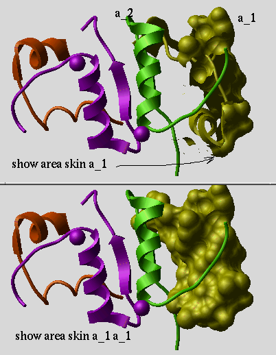
read object s_icmhome+"crn.ob"
set area a_1//* 0. # make sure that the initial area is zero
show surface area a_1//!h* a_1//!h* # only the first molecule
show Area(a_//*) # individual areas, hydrogens have 0.
show Sum(Area(a_//!h*)) # the total
show atoms
show as
shows properties of the selected atoms.
Example:
build string "se ala"
show surface area
show a_//c*
Atom Res Mol Obj X Y Z Occ B MMFF Code Xi Chrg formal Grad Area Grp
The fields:
Field Description
Atom atom name
Res residue number+[symbol] and name
Mol molecule name
Obj object name
X,Y,Z coordinates
Occ occupancy (from 0. to 1.)
B B-factor (positive)
MMFF MMFF atom code
Code ICM atom code
Xi chirality number (0,1,2,3)
Chrg partial charge
formal formal charge
Area solvent accessible surface area
Grp electrostatic group (atoms can not be separated)
as_ selection expression
show atom type
show atom type
show atom type mmff [ { s_pattern | i_type } ]
shows atom types stored in the icm.cod file. The mmff option
allows one to check the Merck Force Field atom type.
Examples:
show atom type
# show all ICM types
-------------{atom codes}-----------
#
# icd vw hb hd wt sf na
#
atcd 0 0 0 0 0.000 0.00 ?
atcd 1 1 1 0 1.008 0.00 h
atcd 2 3 1 0 1.008 0.00 h
...
show atom type mmff "*cation*"
# cations
show atom type mmff "*iron*ion*"
# do we have iron ions?
show atom type mmff "?C=*"
# what types are connected to doubly-bonded carbon ?
show atom type mmff "[!C]*ring*"
# non-carbon types in rings
show atom type mmff 32
# some oxygens
-----------{MMFF atom codes}--------
Symb.Typ.[V] Description {formal charge}
O2CM 32 [1] oxygen in carboxylate anion
OXN 32 [1] N-oxide oxygen
O2N 32 [1] nitro oxygen
O2NO 32 [1] nitro-group oxygen in nitrate
...
show bond : detecting problematic covalent geometry
show bond as [mute|error|]
show clash
show clash [ mute ] [ as_1 [ as_2 ] ] [ -r_vwDistanceFraction ] [ r_distance ]
shows all the interatomic distances between two atom selections which are
shorter than the sum of two van der Waals radii multiplied by the r_vwDistanceFraction
parameter (0.8 by default). This command can be shown to show the short contacts only
if the limit is about 0.8, or show show all pairs of atoms with significant
van der Waals contribution (the limit of about 1.2 )
See also: display clash, undisplay clash.
Visualize the strained atoms with show a_//G or display a_//G .
Example:
build string "se ala his trp glu"
randomize v_//*
display
show clash a_//c* a_//c* # clashes between carbons
show clash a_//c* a_//c* -0.7 # more tolerant test
display clash
show color list
show color [ mute ]
shows list of colors defined in the file icm.clr
and stores the output list in the S_out string array.
Option mute suppresses output to the screen but still
saves to the S_out array (useful for scripts)
See also: color command.
An example:
show color
-------------{colors}-----------
1 black #000000
2 white #ffffff
3 grey #878787
4 blue #0065ff
5 red #ff0000
...
Example of show color mute use in a script:
if (Exist(view)) then # check if graphics is active
show color mute # saves a list of colors in S_out
for i = 1, Nof(S_out)
color background $S_out[i]
pause
endfor
endif
show arrays as parallel vertical columns
show column array1 array2 .... [ s_fileName ] [ separator= s_Separators ] [ comment= s_Comment ]
shows several arrays in a multi- column format.
If you want to shorten the significant digits in real arrays, use this trick:
a = {1.333333 2.44444} # creating some dumb arrays
b = a
show column Rarray(a,2), Rarray(b,1)
See also: write column, show database, write database.
Example:
resnam = {"ala" "glu" "arg"}
reschg = { 0., -1., 1.}
show column resnam reschg
show column separator=":" comment="Example table" resnam reschg
show comp_matrix
show comp_matrix
shows residue comparison matrix
used by the alignment algorithms.
See also: set comp_matrix, read comp_matrix.
show table in database format
show database { table | array1 array2 .... }
shows several arrays or a table in a database format.
See also: read database show column, write database.
Example:
resnam = {"ala" "glu" "arg"}
reschg = { 0., -1., 1.}
show database resnam reschg
show drestraint
show drestraint [ as_select [ as_select ]] [ center ] [ mute ] [ r_violation ]
shows distance restraints.
Arguments:
Output:
See also: drestraint and drestraint type.
show drestraint type
show drestraint types
shows available drestraint types as defined in the icm.rst file.
The numbered global or local types can be used to impose distance restraints.
The other types are fixed and are used to impose disulfide bonds or
peptide bonds.
show energy
show energy [ mute ] [ s_termString ] [ vs ] [ as_select1 [ as_select2 ] ]
calculates and shows values of currently set or explicitly defined in
s_termString energy terms (e.g. "vw,el" )
Important: the boundary element electrostatics is the most
computationally heavy term. It is activated if electrostatic term
el is switched on and preference electroMethod is set to "boundary element" .
The most demanding part is the calculation of the boundary and its characteristics.
Therefore, for multiple calculations with the same boundary we recommend to use
make boundary and delete boundary commands.
show energy atom, crystallographic electron density energies
the result is added the value of 20. and is set to the atomic bfactor field (see Bfactor( as ) and set-factor.
build string "ASD"
make map potential "gp"
show energy atom "gp"
gp_e = Bfactor(a_// ) - 20. # atomic energy contributions, -20 to eleminate shift
add column t Group( gp_e , a_// "sum" ) Name( a_/ ) full) # Group aggreates into residues
show t
loadEDS "3pah" 0. # loads m_3pah crystallographic 2Fo-Fc map for epinephrine
read pdb "3pah" # unconverted pdb
bx = Box( a_aale 5. ) # R_6box around epinephrine
convert Res( a_//* & bx ) # carve out region of interest and convert to ICM
make map potential m_3pah bx # box around epinephrine, makes m_xr
m_g1 = Trim(m_xr, -1., 1.)
set type property {1.} Count(50,300)//Count(330,404) only # without H
set bfactor a_//* 0.
show energy atom "gp"
set bfactor a_//* & bx 20.-Bfactor(a_//* & bx)
Select( a_// "b<0.5") # each atom knows its map value (shifted by 20.)
show energy gradient
show gradient
show gradient calculated by the minimize or show energy commands.
show hbond
show hbond [ mute ] [ as_1 [ as_2 ] ][ r_maxHbondDistance ]
calculates and outputs the list of hydrogen bonds between two atom selections.
By default calculation is done between all the atoms of the current ICM object.
The real argument r_maxHbondDistance defines the upper bound of the
distance between a hydrogen and a potential hydrogen acceptor to place
the pair to the hydrogen bond list. Default value of r_maxHbondDistance
parameter is 2.5 A. Number of identified hydrogen bonds is saved in i_out .
To display/undisplay hydrogen bonds, use display hbond and
undisplay hbond commands.
Hydrogen bonds can also be calculated by the minimize and show energy
commands provided that the hydrogen bond term is switched on.)
show hbond exact : accurate bonding energy calculation
show hbond exact (-1 if atoms are not connected)
calculate the hydrogen bonding energy according to the distributed electron density geometry. Used in virtual screening to
evaluate a score. The calculation builds the lone pair positions at 1.A distance from the acceptor and uses the angular dependent formula to calculated the 'strength'.
The strength of a hydrogen bond is placed in the user ouput field of the donor atom (a single atom)
and is accumulated in the user output field of the acceptor atom (can support multiple hbonds). The field is returned by the
Field(
show table in html format
show html T [format=yes] [frame=1] [chemical=yes] [header=yes] [size=I_chem_size] [view]
show the T_ table with HTML tags.
See also:
Example:
add column t Chemical("CCC")
show html t
show iarray
show iarray
show all integer arrays defined in the shell. Identical to list iarrayIt shows names, dimensions and the first elements of arrays.
The I_out array contains the output of some functions and commands and
is always in the shell.
ii={1 2 3 4 5 6 76}
iii=Count(10)
show iarray
---------------{iarrays}-------------
show integers
show integers
show all integer shell variables.
Example:
show integer
---------------{integers}------------
a 111
autoSavePeriod 10
defSymGroup 1
show label
show labels
show graphics string labels to find out their number. Then the labels
can be addressed as label 1, label 2 etc.
See also: display string_label
show library
show libraries
show loaded ICM-libraries. It's a lot of stuff, enter 'q' to exit.
show link
show link [ ms ]
show links between molecules of 3D molecules and corresponding sequences and alignments.
show logical
show logicals
shows all logical shell variables in ICM-shell.
Example:
aa=yes
show logical
---------------{logicals}------------
aa yes
l_alignProfiles yes
l_antiAlias yes
l_antiAliasGLfix no
l_autoLink yes
l_bpmc yes
...
show mol
show mol as_select
shows selected atoms in the mol file format.
See also: read mol and write mol.
show mol2
show mol2 as_select
shows selected atoms in the mol2 -file format (file extension .ml2).
See also: read mol2 "file" and write mol2 "file" .
show molecule
show molecules
shows all molecules of all objects currently in icm-shell.
This command is identical to show a_*.*
show object
show objects
shows all molecular objects currently in icm-shell. This command is
identical to
show a_*.
The same result is achieved with the
list a_*. command.
show pdb
show pdb as_select
show selected atoms in the PDB file format.
See also: read pdb "file", and write pdb "file".
show pmf
show preferences
show preference
shows all icm preference variables in icm-shell (e.g.
show preferences
..
atomSingleStyle = "tetrahedron"
1 = "tetrahedron" # current choice
2 = "cross"
3 = "dot"
..
show profile,rarray,real,sarray,string
show profile | rarray | real | sarray | string
shows all objects of specified type(s) in icm-shell. E.g.
E.g.
show sarray rarray
show residue
show residues
shows all residues in all molecules of all molecular objects.
This command is equivalent to
show a_*.*/*
show residue type
show residue types
shows names and characteristics of compounds described in the icm.res and user ICM residue libraries.
show segment
show segment [ ms ]
show segment representation of 3D structure of a protein for the
selected molecules ms_ (all molecules of the current object by default).
See also assign sstructure segment,
ribbonStyle, display ribbon.
show sequence
show sequences [selection] [ number ] [ { fasta | swiss | pir | gcg | msf } ]
show all sequences or the specified sequence seq_ in one of specified formats.
The default format is the fasta format.
Option number defines if the residue numbers are added.
Option selection only shows sequences selected graphically or with the select sequence .. command
Three logicals: l_showSstructure, l_showSites, and l_showAccessibility
control the display of a corresponding additional information aligned with the sequence.
Example:
readUniprot "RXRA_HUMAN"
show sequence swiss RXRA_HUMAN
read pdb "1lbd"
show surface area
make sequence
Info> sequence 1lbd_a extracted
show 1lbd_a # you see relative accessibilities in 0-9 scale
l_showAccessibility = no
show 1lbd_a
show stack
show stack [ [ i_FromConf ] i_ToConf ]
show the following parameters of the conformations currently residing in the conformational stack.
show table
show [ table header ] table [database] [compress]
shows the specified table in the ICM table format (one line per table row)
or ICM database format (a list of column-name column values pairs for each
entry).
Options:
add column t 2.22222//3.33333 1//2
set format t.A "%.2f" # two digits after .
show t compress
add column t {1.333333 2.44444} # creating some dumb table with one column
t.A = Rarray(t.A 2) # will trim to 2 sign digits
show t
See also: show html T_ .
Database index tables are exceptions, show T_index will show all the entries
of the related database. To see members of an index table type the index table
name and press TAB.
show terms
show terms [ all ]
shows the active energy/penalty terms. With option all it shows all the terms available.
The result is saved in the s_out string.
You can also use the Info (term) function to return
the term string.
See also: set terms, Info (term), delete terms.
show tethers
show tethers [ mute ] [ as_select ] [ r_minDeviation ]
Shows tethered atoms with deviation larger than r_minDeviation
(0. by default) and returns these atoms in as_out .
Option mute is used when you just want to get a selection (as_out)
of strongly deviated atoms.
See also: display tethers.
show a full Uniprot entry
show uniprot_index_table_name.ID == s_uniprot_ID [ output=s_string_var_name l_info=no ]
read index "/data/uniprot/sprot.inx" #creates sprot index-table
show sprot.ID == "IL2_HUMAN" output="up_text" l_info=no
write up_text "il2.txt"
show version
show version
show characteristics of the current ICM executable. Part of this string containing
the version number is returned by the Version( )
function.
show vrestraints
show vrestraint [ vs ]
shows vrestraints imposed on the internal variables of ICM molecular object.
show vrestraint type
show vrestraint types
shows types of vrestraints. These types are loaded from the icm.rst file.
show volume
show volume skin [ mute ] [ as ]
Calculates the volume confined by the solvent-accessible surface
or molecular surface (so called "skin"), respectively
. One optional selection as_1 defines atoms for which the volume is calculated.
If the selection is not specified, the atoms are assumed to belong to the current object.
The volume will be stored in r_out and the number of triangles used in the
skin construction in i_out .
Examples:
read obj s_icmhome+"crn.ob"
show volume surface # inside accessible surface
print "volume inside accessible surface = ", r_out
show volume skin # inside molecular surface
print "volume inside molecular surface = ", r_out
calculate volume of blobs of map density.
show volume [ map ] [ I_indexBox[1:6] ] [ r_Threshold ]
Contour electron density map at a given r_Threshold and
calculate the volume of the high-density blobs. Defaults:
Threshold is expressed in the units of standard deviations from the mean
map value, i.e. 1. stands one sigma over the mean.
The volume will be stored in r_out .
See also: make grob m_ .
Examples:
read map s_icmhome+"crn.map" # load m_crn map
show volume m_crn 3. # calculate volume inside the
show supported pharmacophore types
sort
sort array(s)
sort one or several integer, real or string arrays. The first array is
the sort key. By default ordering is lexicographic for string arrays and
by increasing arithmetic value for integer and real arrays.
Options:
See also: Sort .
Examples:
a={3 2 1 5 7 4 6}
b=Sin(a*50.)
c={"three" "two" "one" "Five" "Seven" "four" "Six" }
show column a b c
sort a b c
show column a b c
sort reverse b a c
show column a b c
sort c b a
show column a b c
sort table
sort [ reverse ] [ number ] [ history ] table.keyArray1 [ reverse ] table.keyarray1 [ reverse ] ...
this command sorts all the arrays of the table so that all the listed table.keyArrays
are applied sequentially with descending priority.
Each array can be followed by the reverse option to change the sorting order.
Examples:
read table s_icmhome+"res.tab" # residue properties
RES = $s_out # create an ICM table RES
sort RES.aa # resort entries by residue name
show RES
sort reverse RES.flexInd RES.aa
show RES
sort RES.hPhobInd RES.flexInd
show RES
sort table column
this command sorts table columns by column names (the default) or by custom function/expression.
Examples:
makeTable "t" 10 0 0 3 no no no yes
sort column t function="Icm::Min(COL)" # Sorts by minimum value ('COL' refers to the current current column)
sort column t name={"B","C"} function="Icm::Corr(COL,A)" reverse # Sorts columns 'B' 'C' by correlation to column A
# select columns first then sort the selection
add column t 'john'//'jack'//'mike' 2.//4.//2. 3.//5.//2. 6.//7..//8.
select column t rarray # leaves non-numeric columns alone
sort column t selection function="Icm::Mean(COL)" reverse
# takes a mean of each column and sorts column by that mean
sort and reorder molecular objects
sort object os_ i_pos
# move selected objects to a give position
resorts all molecular objects by the specified user field
(see the set field command, and the Field function). If the field
is not specified, the objects are sorted by their mass.
sort molecules in an object by mass or a user field
sort os_ObjectSelection [ field = i_Field ]
resorts the molecules in each of the selected non-ICM objects by the specified user field
(see the set field command, and the Field function). If the field
is not specified, the molecules are sorted by molecular mass.
An ICM object can be stripped, resorted and then converted again.
Sorting a stack of conformations
sort stack
sorts conformations in a stack according to their energies.
New energies can be assigned to the same conformations with the set stack energy command.
split
split grob
split g_complexGrob [ s_rootGrobsName] [ i_maxNofGrobs] [ r_minNofPointsInGrob ]
divides disconnected parts of a graphics object into a bunch of separate graphics
object sorted according to their size (measured as the number of vertices).
The maximal number of new grobs is defined either by i_maxNofGrobs
explicitly or by the MnGrobs parameter.
The latter can be redefined in the icm.cfg configuration file.
The i_maxNofGrobs option allows one to retain only larger pieces.
Grobs will be sorted according to their number of points and
named by adding their sequential number to the input grob name or s_rootGrobsName, if specified.
The split command is used in protein cavity analysis and other applications where
one needs to treat, display, and measure disconnected parts separately.
You can also limit the number of points of the grobs generated by the command by providing
the real argument with the minimal number of vertices you want in a grob.
See also: Volume( g_), Area( g_), Xyz( g_).
Examples:
read object s_icmhome + "crn"
make grob skin a_//cb a_//cb name="g_crn"
split g_crn
display grob smooth # display as one smooth surface
undisplay g_crn
color grob unique
show Volume(g_crn3) Area(g_crn3)
read map s_icmhome + "crn"
make grob
split g_crn "blob" 30 # create up to 30 largest grobs and
# call them "blob1" "blob2"...
# a variant: split g_crn "blob" 40 100.0 # discard grobs smaller than 100. vertices
delete g_crn
display grob
color grob unique
ball1 = Grob( "SPHERE" , 1. , 10 ) + {0. 0. 0.} # ball is centered in {0. 0. 0.}
split ball1 Matrix( { 0. 0. 0. 1. 0. 0. 0. 1. 0. } 3 ) # splits by XY plane
display ball1_1
display ball1_2
split group : derive replacement group arrays from a combinatorial library and a scaffold.
Output:
smi = {"C1CCC2C(C1)CCCN2", "CCC1CCCNC1C1CCCCC1", "CC1CCCNC1C1CCCCC1", "C1CCC(CC1)C1CCCCN1"}
add column t Chemical( smi )
split group t.mol Chemical( "C1CC(C(NC1)[R2,H])[R1,H]" ) name="tt"
Splitting a table to column arrays
split T_table_with_more_than_one_column
split the table into individual arrays with the names corresponding to the names of table columns (e.g. A, B). If the operation is successful the source table will be deleted after the array generation.
Example:
add column t {1 2 3} {22 33 44} name={"aa","bb"} # t.aa t.bb arrays
split t # aa and bb arrays and t is deleted
Splitting a sequence to domains between NNN. runs
a=Sequence("AAANNAAAAAAAAAAAAAANNNNNNAAAAAAAAANANA" nucleotide )
split a 3
show sequence
Splitting multiple values in each cell of a column into single-value cells by multiplying rows.
split [ tableColumn ] [ separator= character ]
For sarray column takes each string of the specified column and splits it by the separator
(comma is the default separator, e.g. separator="," )
The rows are multiplied accordingly. Example:
group table t {1,2} {"a,b,c","d,e"}
t
#>-A-----------B----------
1 a,b,c
2 d,e
split t.B separator=","
t
#>-A-----------B----------
1 a
2 d
1 b
1 c
2 e
Note that extra columns are appended to the original table (that explains somewhat strange order).
# group conformers by MOL_NUM aggregating conformations into stack
group conformers.MOL_NUM conformers.mol "conf_concat," all "first" header name="conformers_stack"
# split back
split conformers_stack.mol
Splitting an object into separate molecules
split object
There is no such command, however there are two useful ICM-shell macros that you may call.
read pdb "3fuc"
splitByChain a_ yes yes no # you get three objects with individual chains and delete the original one
copy a_ "b"
delete a_b.!1 # delete all but the first molecule
write a_b. "b" # contains only the first molecule
#
copy a_ "c"
delete a_c.!2 # delete all but the second molecule
write a_c. "c" # contains only the second molecule
#etc..
Changing the position of tree cursor (separator) and calculating new cluster numbers
split T.cluster 1 0.14 # take the 1st tree and set distance threshold to 0.14
sprintf
sprintf [ append ] s_formatString arg1 arg1 arg2 arg3 ... [ name= s_outputStringName]
Print to the s_out string, or the s_outputStringName specified
after the name= option.
The same syntax as printf command, but the result is not displayed.
Example in which string outStr is the destination:
sprintf "mncalls = %d\n",mncalls name="outStr"
store
store conf
store conf [ i_slotNumber ] [ os_obj ] [s_comment]
store current conformation into specified slot of the conformational stack.
By default it puts the conformation into the first free slot, or appends it to the end.
The energy, by default, is automatically extracted from the previous energy evaluation,
or taken from r_energy if explicitly provided. The total number of visits ( nvi ) is set to
1 by default.
build string "WSD"
montecarlo # generates a stack
show stack
set v_//omg 180. # change a conformation
store conf -9. "mycomment" # add conformation with energy -9. and comment string
store conf 3, -9. # override slot 3 with energy -99.
store conf number=33 # set conf with number of visits=33
See also set stack property array_of_values command , e.g.
set stack energy Random(0., 10., Nof(stack))
for multiple assignments of energy values, number of visits or total number of visits.
store conformational stack inside an object
store frame
The advantage of the trajectory file is the possibility of interpolated display as a trajectory animation.
See display trajectory .
for i=1,Nof(conf)
load conf i
store frame
endfor
store frame write
#
display ribbon
display trajectory sstructure 20. 40.
ssearch
is a systematic search through torsion
space combined with local minimization.
ssearch [ local ] [ residue ] [ vs_Ssearch [ vs_minimize ]] [ as_select1 [ as_select2 ]]
systematically changes vs_Ssearch variables and carries out
energy minimization with respect to the vs_minimize variables
after each systematic conformational change.
The lowest energy conformation is loaded from the conformational stack at the end of the procedure.
By default every variable from vs_Ssearch selection goes through nSsearchStep evenly distributed values.
The step therefore is 360 deg. over nSsearchStep.
Option local imposes the grid locally around the current values of vs_Ssearch variables.
In this case the program uses ssearchStep parameter.
If you want to prevent the procedure from automatically writing
the stack of best conformations to a file
set the autoSavePeriod variable to zero.
See also montecarlo .
Example:
read object "crn" # good old crambin
ssearch v_/14/x* # place optimally Asn14 side-chain
ssearch residue v_/tyr/x* # loops through tyrosines and ssearch each separately/
# ssearch residue simple vs_ # GAP model only
strip
strip os_object [ virtual ]
strip an ICM-molecular object from its ICM attributes and reduce it into
a pdb-object. The latter are still good for graphics, superposition,
basic geometric manipulations etc. Also, some chemical operations,
e.g. attaching chemical groups are best performed on simpler pdb-objects.
Stripping may save you a lot of memory as well.
Option virtual tells the command to delete the virtual atoms upon conversion.
The virtual atoms ( selected as a_//vt* ) are always present in the ICM object,
but are not necessary in the stripped object.
String is also used to perform operations which are not allowed for
ICM object, but are allowed for simpler PDB objects (for example
dragging individual atoms with a mouse)
These commands include:
After you have done editing the stripped (non-ICM) object, you may convert it back to a fully functional one by the convert command it its simplest form (do not need a convertObject macro)
Example:
build smiles "c1ccccc1"
strip a_ virtual
superimpose
superimpose [ [ align | residue | ali ] [ exact ] [minimize] ] as_selectStatic as_selectMovable
superimpose os_static I_atomNumbers1 os_movable I_atomNumbers2
superimpose as_movableByTethers [ reverse ]
optimally superimpose the second movable object onto the first one using selected atoms or
residues as equivalent points. At least one pair of equivalent atoms needs to be
provided.
The second molecule can also have a selection, then the intersect of the two selections will
be used for superposition.
read pdb "1ql6"
read pdb "2phk"
make sequence a_*.1
Sequence(a_*.1)
alig = Align( 1ql6_a 2phk_a )
Edit this alignment if necessary (usually you do not need to do it)
bindpock = Sphere( a_2phk.atp a_2phk.a 10. )
superimpoase bindpock a_1ql6.a alig
If you do not care about the alignment, it can also be generated on the fly with the align option
instead of the alignment name.
alignment options:
Number of equivalent atom pairs is saved in i_out; resulting RMSD is saved in
r_out; a selection of atoms in the "static" object used for superposition is
saved in as_out, that of "movable" object in as2_out .
Virtual atoms. Be default, the first two virtual atoms ( vt1 and vt2 ) are automatically
excluded from both selections unless the virtual option is explicitly specified.
Note that if the movable object is of ICM-type it is preferable to have all six
virtual variables unfixed ( e.g. unfix V_movableObj.//?vt* ).
Otherwise, if some or all of them ( V_//?vt* ) are fixed, you will get
a warning, and only the partial minimization of the RMS distance possible
with the given degrees of freedom will be performed.
If the explicit order of atoms is specified and two single object selections
are provided, e.g.
superimpose a_a. a_b. {3 5 7} {10 3 5}
the superposition will be performed in the specified order.
The following output is produced:
Iterative search of the best atom pair subset for superposition.
sys (or unix): system command
sys system_shell_command
unix unix_shell_command
issues a system shell command from ICM. You may use sys or unix
interchangeably. However, every time your ICM script makes a system call, ICM spawns a new process.
Keep in mind that some simple external operations on files and directories are possible without the thread-spawning unix command. Here is the list of what can be done without it:
command comment unix equivalent example
delete system s_file delete a single file rm file a="1crn.ob"; delete system a
rename system s_f1 s_newname rename/move a single file mv file1 file2 rename system "1crn.ob" "1crn_old.ob"
copy-systems_f1 s_f2 copy a single file cp file1 file2 copy system "a" "b"
set directory s_dirname change directory (cd) cd dirname set directory "./DOCK1"
make directory s_dirname make a directory mkdir make directory "NEW"
Path ( directory ) returns the path to the current directory pwd s_currDir = Path(directory)
Sarray ( s_filename_filter directory [ all ] ) returns the file list array, all goes to subdirectories ls -1 [-R] name_pattern a = Sarray("*.icb" directory)
if ( <condition> ) sys system_command
is illegal. Use
if ( <condition> ) then
sys system_command
endif
instead.
For cross-platform compatibility, also use the following portable
ICM shell variables instead of non-portable system-specific commands:
s_sysCp , s_sysLs , s_sysLtt , s_sysMv , s_sysRm.
Example:
sys $s_sysLs # cross-platform portable list command
sys ls # non-portable unix only ls command
As you might have guessed from the above example,
to pass the ICM-shell variables to the system_shell_command
one may use integer, real or string ICM-shell variables,
protected with dollar sign ($) prefix.
Important: passing ICM-shell variables to the UNIX command is impossible if you use an alias name
(e.g. ux) instead of the original unix command.
Examples:
unix grep -i myoglobin /data/pdb/brookdir.doc
unix echo $mncalls $s_pdbDir $dielConst
file="/data/pdb/"+Name(a_1.) # tricky file name
unix grep ATOM $file | wc -l # $file will be substituted by
# the value of this ICM-shell
# string variable
test
test yes
test no
test 2==2
test 2==3
test real {2. 4.} 2.*{1. 2.}
test exact {2 4} 2*{1 2}
test binary
then
is one of the ICM flow control
statements, used to perform conditional statements.
See also if, elseif, and endif .
transform
transform string arrays in place
read table s_userDir + "inx/PDB.tab"
transform sarray PDB.head "tolower" # in place
transform molecular objects or grobs
transform {ms|g_grob} R_12transformationVector
See also these two examples: ( example 1 and example 2).
You can also manually move molecules with respect to each other on the graphics screen by using the
connect ms_ command to choose the molecules which can be moved separately.
transform ms i_transformationNumber [ translate [= <{x,y,z}> ] ]
transform molecules ms_ according to the specified transformation.
i_transformationNumber is a symmetry operation number in an array of all operators of
a space group. The first transformation usually keeps the object in place.
The symmetry transformations are defined in a 12*n real array where
each chunk of 12 real values defines 3x3 rotation matrix and translation
vector {a4,a8,a12}. The complete 4x4 transformation matrix looks like this:
a1 a2 a3 | a4
a5 a6 a7 | a8
a9 a10 a11 | a12
------------+----
0. 0. 0. | 1.
Example:
read pdb "1sre"
copy a_1. "a1"
transform a_a1. Transform(a_a1.)[13:24] # Trasform with R_12transformationVector
copy a_1. "a2"
transform a_a2. 3 # same using i_transformationNumber
translate
translate { os | ms | g_grob .. | origin } { add R3_transl_vector | R3_destinationPoint | M_xyz [symmetry]
translate the center of mass of the specified object(s) ( os_ ) or molecule(s)
( ms_ ) to a specified position, or, with the add option, by a R_3translationVector vector.
If a Nx3 matrix is specified, the mean vector is calculated.
You can also move molecules/objects interactively with the mouse after the connect command.
Without the add option, the translation
symmetry option With the symmetry option the R_3translationVector should be in fractional coordinates.
Option add translates by the specified vector from the current position.
Without add the program tries to identify a compensating shift to a position in which
the center of gravity of the selected molecule(s) has minimal positive fractional coordinates.
Examples:
read pdb "1fbi"
delete a_!p,q,y # get rid of redundancies
copy a_ "a1"
translate a_a1. add symmetry {0., 0., -1.} # shift whole object by fractional coordinates
cool a_
for i=1,10
translate a_y add {0., 0., 0.9} # shift molecule y by an increment
endfor
To calculate a displacement vector, follow this example in which we calculate
a translation vector for molecule y :
read pdb "1fbi"
delete a_!p,q,y # get rid of reduncancies
cool a_
v1 = Rarray( Xyz( a_y/1/ca ) )
connect a_y # now drag the molecule with the middle button and press Esc
v2 = Rarray( Xyz( a_y/1/ca ) )
vtrans = v2 - v1
undisplay
undisplay [[ms] store] args
Opposite to display .
Examples of the undisplay command:
undisplay store a_1,2 # undisplay the two molecules and memorize their appearence
undisplay ribbon # ribbon display not needed any more
undisplay g_icos # a graphics object not needed any more
undisplay a_/w*,hoh* # who cares about water molecules ...
undisplay residue labels # just "labels" will do the same
undisplay string # see also "delete label" command
undisplay a_//h* # who cares about hydrogens ...
undisplay hbond a_1./1:29 # ... and, hence, about H-bonds
undisplay tether a_/12:20
undisplay box
undisplay cursor
undisplay origin # undisplay the coordinate frame
undisplay volume # deactivate the fog effect
undisplay window
To get rid of the whole graphics window for fast calculations use:
undisplay window # delete GL graphics window
undisplay window
unfix
unfix [ only ] Vs_select
unfix (set free) specified variables (such as bond lengths, angles and
phases or torsions) in an ICM-object. Opposite to fix command.
This operation can be applied to the current object
only (use set object os_newObj first).
Important: since it only makes sense to unfix variables which
are currently fixed, use all variable selection starting with capital V
which selects among ALL (both free and fixed) variables,
as opposed to vs_ which selects only from FREE variables.
Examples:
# only this loop has free torsions now
unfix only V_/8:18/phi,PSI,H,M,P
Note that PSI torsion references is used for traditional residue attribution
wait
wait for the child ICM processes to finish, quit the child processes
wait [pipe]
allows one to synchronize multiple ICM processes spawned by the fork command.
web
s_ncbi= "http://www.ncbi.nlm.nih.gov/entrez/viewer.fcgi?db=protein&val="
web s_ncbi+"Q28509"
web table: shows an icm table with a web browser
web [ delete ] [ s_file] T [ link T.S_1 s_linktype1 T.S_2 s_linktype2 ... ]
The command presents the T_ table in your web browser window. Optional web links are
interpreted according to the web link types described in the WEBLINK.DB array.
If the table contains chemicals, ICM creates a file with the compound images using
Peter Ertl's JME classes (see also the s_javaCodeBase variable).
Example:
read sequence "zincFing.seq"
find prosite 1znf_m 0.3
show SITES
web SITES link SITES.AC "AUTO"
while
while
is one of the ICM flow control statements, used to perform a loop
in the ICM-shell calculations.
See also: for, endwhile .
write
For the list of ICM-objects you can write, and formats you can choose, see read and show commands.
Generic syntax:
write [binary] [ append | delete ] { variable | constant | expression } s_fileNameRoot[.ext]
With the binary binary option multiple objects or classes of objects can be writtin into
a single cross-platform compatible binary file. To read it use read binary and to read the
table of its contents use read binary list .
See also corresponding read commands.
write alignment
write [ alignment ] [ msf | fasta ] ali_Name [ s_fileName] [ SEQUENCE.restoreOrigNames=yes|no ]
write alignment ali_Name to a file. Default extension is .ali .
Note: if alignment is only a group of unaligned sequences,
generated by the group command, the result will be just a
multiple sequence file, rather than an alignment file
(there will be no dashes at the end).
The default ICM format for an alignment looks like this:
#>ali sh3
# Consensus ...#.^.YD%..+~..-#~# K~-.#~##.~~..~WW.#. ~~.~
Fyn ----VTLFVALYDYEARTEDDLSFHKGEKFQILNSSEGDWWEARSLTTGET
Spec DETGKELVLALYDYQEKSPREVTMKKGDILTLLNSTNKDWWKVE--VNDRQ
Eps8 KTQPKKYAKSKYDFVARNSSELSM-KDDVLELILDDRRQWWKVR---NSGD
#Fyn __EEEE__________________EEEEEEE____EEEEEE_____E
# Consensus G%#P...#..#.
Fyn GYIPSNYVAPVDSIQ
Spec GFVPAAYVKKLD---
Eps8 GFVPNNILDIMRTPE
#Fyn EEEGGGGEEE_____
# nID 7 Lmin 61 ID 11.5 %
The lines starting from hash (#) are comments and are not required
The length of each alignment block is controlled by the sequenceLine parameter (default value is 60).
If you want to save a long alignment as one unwrapped block,
increase this value (e.g. sequenceLine=1000 )
Writing sequences in the alignment order
The sequences can be written in the alignment order with the following commands
(they can be store in a little macro)
macro wrSeqAli ali_ s_file ("seq.fasta")
l_showSstructure = no
seqname = Name(ali_) # Name returns sarray of sequence names
for i=1,Nof(seqname)
write sequence fasta append $seqname[i] s_file
endfor
endmacro
Resorting alignment in the order of sequence input.
Upon alignment the source sequences get reordered according to similarity.
If you want to keep the original order you may use the reorderAlignmentSeq macro
described in the Align( ali_ I_newOrder ) section
and then write an alignment:
read sequence s_icmhome+"zincFing"
group sequence aaa
align aaa
reorderAlignmentSeq aaa
write ali_new # reordered alignment
See also: SEQUENCE.restoreOrigNames , String( ali_) function.
write binary
write binary [ class1 class2 ... ] [ os_objects [tether] obj1 obj2 ... ] [ s_fileName |stdout ]
write specified ICM shell objects or all objects of a classes to a
single, binary, cross-platform file, or more accurately, database.
The following data types are currently supported:
The default file name is "icm.icb", and the default extension is
.icb (stands for ICm Binary file).
The system objects or the objects with property
h4-- Making a table of content of any icb file, and reading only certain ICM objects
The catalogue of the database can be obtained with the list binary command.
The same list can be extracted into a table with names one can use to extract only objects of interest from an .icb file. E.g.
list binary "myfile.icb" name="Toc" # just look at it in ICM terminal
read binary list "myfile.icb" name="Toc" #extract to table named Toc (.name, .type, .size)
read binary "myfile.icb" name="7cpu" # if you see it in the file
# or
read binary "myfile.icb" name={"1crn","7cpu"}
* --all save all objects in the shell (system variables are skipped)
* --key= ~~s_password protect the file with a password. To open this file with the password, use the File menu ( Open with password)
From the command line: to open a protected file, use
read binary [all]
Examples:
ii = {2 3 4}
rr = {2. 3.4 5.5}
g = Grob("CELL",{1. 1. 1.})
g2 = g*2. # twice as large
write binary iarray rarray grob # the default file is icm.icb
Info> 4 icm shell objects icm.icb
list binary # looks at "icm.icb"
1 ii iarray 20
2 rr rarray 32
3 g grob 1788
4 g2 grob 1788
delete ii
read binary name={"ii"}
Info> 1 icm shell objects read from icm.icb
write binary grob "aaa"
Info> 2 icm shell objects aaa.icb
See also: list binary, read binary
write iarray
write [ iarray ] I_name [ s_fileName ]
write rarray
write [ rarray] R_name [ s_fileName ]
write sarray
write [ sarray] S_name [ s_fileName ]
write matrix
write [ matrix ] M_name [ s_fileName ]
write an array or a matrix to a file. Default file extensions are
.iar, .rar, .sar, or .mat, respectively.
See also:
read iarray,
read rarray,
read sarray,
read matrix.
write molcart
write several arrays
write [ { column | database ] } array1 array2 .... [ s_fileName ]
write arrays in the column or database format to a file.
Default file extension is .db
See also: read database.
writing tethers
If you imposed tethers between you current object and another object and you want to
quit the session and then restore you setup, you can use the following trick:
# first let us create an object a_ly6. tethered to template a_x.
read alignment s_icmhome+"sx"
read pdb s_icmhome+"x"
build model ly6 a_x.m # a new object a_ly6. created and tethered
#
write string String( a_//T ) "tTz.str" # tethered model atoms
write string String( a_//Z ) "xTz.str" # x-template atoms
write object a_x,ly6. "tx.ob"
#
quit
#
% icm
read object "tx.ob"
read string "tTz.str" name="tTz"
read string "xTz.str" name="xTz"
set tether $xTz $tTz exact # tethers restored
write table
writing ICM table in text format write T_table1 [ T_table2 .. ] [header] [ separator=s_delimiter | csv ] [ s_fileName or s_file.xlsx ] [number] [compress]
write the T_table1,.., tables to a file in several formats depending on the the s_delimiter and/or the filename extension (e.g. for the excel .xlsx files).
Output file types:
Example:
group table t {1 2 3} "a" {"one","two","three"} "b"
t1=t[2:3]
write t t1 "tt" # write both tables in one file
write t "tt.xlsx" # write table into an excel file
write t csv "tt.csv" # write table into a comma-separated file
delete table # read both tables
writing tables in a binary format
write binary T_table1 T_table2 .. s_file
The most compact and fast format is the binary format.
Any object can be saved to and read from a binary project file with ".icb"
(ICM-binary) extension.
See also write database T and write column.
Writing/exporting an sdf/mol file
writes an ICM chemical spreadsheet as a mol/sdf file.
All the property columns are added as feature records to individual mol-entries.
Options:
Example:
read table mol "ex_mol.mol" name="t" unique
write table mol t
write T_table1 [ header | number ] [ separator= s_delimiter ] [ s_fileName ]
if the separator or the s_fieldDelimiter variable contain just
a simple symbol (e.g. comma or tab), ICM will
write a comma-separated or tab-separated table with the first line containing
the field names, e.g.
group table t {1 2 3} "a" {"one","two","three"} "b"
write t header separator="," "t.csv"
unix cat t.csv
a,b
1,one
2,two
3,three
write t separator="," "t.csv" # without header
unix cat t.csv
1,one
2,two
3,three
Option compress imposes user format for arrays of real values. The format may be assigned to a column by the set format col command. Example:
delete t
add column t 1//2 3.3333//4.44444 # creates 'A' and 'B'
set format t.B "%.1f"
write t separator="," compress "/tmp/t.csv" # will write 3.3//4.4
read table separator="," header name="t" "t.csv"
write column
write column array1 array2 .... [ s_fileName ] [ separator= s_Separators]
write arrays in a multi- column format to a file.
Examples:
read column s_icmhome + "res.tab" # amino acid properties
write column aa flexInd "tm.tab" # two columns
If you want to write all the entries of an ICM-table you may do the following.
Examples:
read column s_icmhome + "res.tab" # a set of isolated arrays
group table RES $s_out # create an ICM-table RES (s_out : array names)
write RES # write in the 'table' layout
write database RES # write table RES in the 'database' layout
Default file extension is .col.
See also:
read column,
show column.
read table,
show table.
write database
write database [ html ] { array1 array2 .... | table } [ s_fileNameRoot ]
write several arrays or a table in a database format to a file
(usually tables are written in a multi column format).
This command can also be used to save a subset of arrays of a table in a specific
order. Option html writes the table with appropriate HTML tags.
See also
read database
write table,
show database.
Example:
resnam = {"ala" "glu" "arg"}
reschg = { 0., -1., 1.}
write database resnam reschg "a" # default extension ".db" will be added
#
group table t resnam reschg
write database t.reschg t.resnam "a" # reverse the order</tt>
write drestraint
write drestraint [ as ] [ s_fileNameRoot ]
write distance restraints of the current object to a file.
See also: drestraints and drestraint types.
write drestraint type
write drestraint types
write drestraint types to a file.
You may define your own types with the set drestraint type
command or by editing a *.cnt file.
write factor
write [ factor ] factor_Name [ s_factorFileNameRoot ]
writes crystallographic structure factors to a file.
write gamess
write grob
write grob off g_name [s_fileName]
write {grob | g_name} [s_fileName] [ append ]
Write/append to a file.
If g_name is not specified, all grobs are written. Depending on
object features, they may be exported in OFF or Wavefront OBJ file formats.
write html
write html T [format=yes] [frame=1] [chemical=yes]
writes the T_ table with HTML tags to a file.
findPubchem "aspirin" no no 100
write html pubchem_hits "pubhchem_hits.html" format = yes header = yes frame = 1 chemical = yes view size = 200 // 150
See also:
write image
write image [png|targa|cmyk|gif|rgb] [display] [print] [postscript [print|preview]] [compress] [stereo] [color|bw] [window=I_xyPixelSizes] [store] [s_fileName]
nice "1crn" # resize the image
delete label
IMAGE.compress = no #just a plain uncompressed image
write image window={4000,2700} # for slides
write image window=2*View(window) # double the res.
IMAGE.generateAlpha logical variable controls if the alpha channel information is added to the SGI
rgb and tif image files. This additional channel describes
opacity of the image pixels and makes the background transparent.
Images generated with alpha channel can be nicely superimposed in the
IRIX showcase since their backgrounds are transparent.
Examples:
display a_1crn. ribbon
write image "a" # a.tif image - about 1400 kB
write image "p" compress # p.tif image - about 88 kB
write image postscript stereo display "aaa.eps"
write image 2*View(window) # hi-res, may screw up labels
unix lp -c a.eps # print if you like the result
See also: write grob, write png - a different version of the png writer: does not allow arbitrary resolution, but allows transparent background, write postscript.
write 2D image
nice "1crn"
# make 3 images with default names and add them to the default album 'album'
make image
make image
make image
write image album[1] "myimage.png"
write image album[1:2] {"img1.png","img2.png"} #specify names to be used
write image album s_tempDir #save all images into the s_tempDir
write 2D chemical image in .png or .svg format
You can increase resolution by adjusting IMAGE.bondLength2D and/or the window argument.
write image Chemical("C(c1ccc(cc1)C(c1ccc(C#N)cc1)n1cncn1)#N") "xxx.svg" IMAGE.lineWidth2D = 1.8 IMAGE.font = "28px bold Arial"
write image t.mol[1] IMAGE.lineWidth2D=3 display="HSA" "/tmp/mol1.svg"
write image Chemical("CCO") "ethanol.png" IMAGE.bondLength2D = 0.8
write image Chemical({"C1CCN(CC1)c1ccccc1", "CCN(C)c1ccccc1" }) display="AR" # aromatic rings + color square instead atom labels
write alignment image
S_al = Name( alignment )
for i=1,Nof(S_al)
s_al = S_al[i]
set property $s_al 2048 # turn on the profile
write image $s_al Name(s_al) + ".png" 4 delete # write high-res (x4) png image
endfor
write index
General text and specialized content (e.g. write index mol) index files.
write index "/tmp/huge.sdf" pattern="" add="$$$$" # file huge.inx will be saved
# alternatively: write index mol "/tmp/huge.sdf"
calculate and write index for a database file described by the control table T_dbDescription,
or by the s_inputFile in the short form of this command.
write index mol "/data/nci.sdf" "nci.inx" # creates nci.inx file
show i_out
read index "nci" name="x" # creates internal index table x
Path(x) # returns /data/nci/
read table x[1:100] # load first 100 molecules to ICM
After the header there is a string array containing the list of fields. To create this table
either define it in a file or use the group table command.
All text fields (except data) are hashed for fast searching.
Example:
write index mol "drugs.sdf" # the index file is saved to the current directory
read index "drugs"
write index mol "./drugs.sdf"
group table t {"ID","DE","KW","SQ"} "fd" header "/data/swissprot/" \
"DIR" {"sprot"} "FI" ".dat" "EXT"
# we created control table t
write index swiss t "/data/icm/inx/SWISS.inx" # make index and save to a file
read index "/data/icm/inx/SWISS.inx" # read index
show SWISS[2:5]
show SWISS.ID=={"12AH_CLOS4","1431_LYCES","B3AT_CHICK"} output="uniprot3" l_info=no #saves entry into a variable
show SWISS.ID=={"12AH_CLOS4","1431_LYCES","B3AT_CHICK"}
read sequence SWISS.DE=="DNA-BINDING"
read index "/data/uniprot/sprot.inx" #creates sprot index-table
show sprot.ID == "IL2_HUMAN" output="up_text" l_info=no
write up_text "il2.txt"
write index blast
write index sequence s_blastRootFileName
create a set of blast-formatted binary files for searches with the
find database command. The command will use all the sequences
currently loaded into the ICM-shell and will create the following compact binary files
(the first three files are the same as those generated by the setdb
blast command):
The relative solvent areas file is saved only if the sequence was generated
from an object in which the areas had been calculated with the
show area surface command. If the .psa file is present,
ICM will modulate the scores with the accessibilities (it will be
more permissive for the accessible residues).
find database write s_DBpath output= s_fastaFile
command.
Simple example (indexing can also be done with the blast setdb routine):
# copy to the current directory and edit the icm.cfg file
# make sure that MnSequences is larger than the number of
# sequences in your database
#
read sequence "fak.seq" # fasta formatted
write index sequence "/tmp/db1"
delete sequences
a=Sequence("MERTDITMKH KLGGGQYGEV YEGVWKKYSL TVAVKTLKED TMEVEEFLKE")
find database a "/tmp/db1" 0.001
formatdb -i /data/blast/dbf/FASTA/pdbaa -n /tmp/p_db
./icm
read sequence swiss web "10KD_VIGUN"
find database fast=10 10KD_VIGUN "/tmp/p_db"
write library
write library [ append ] [ auto ] as_entryAtom [ exit= as_exitAtom] s_libFileRoot
save a selected molecule, residue or a fragment as an ICM-library entry.
Use
set charge,
set bond type and, possibly,
build hydrogens before writing an entry.
We recommend you to do this operation in an interactive session:
display your molecule and Ctrl-Click the first and last atoms
if needed. There are two different situations:
read sequence "aaa.seq"
Example:
build string "nter glu cooh" # build glutamic acid residue
strip # convert it to a non-ICM object
write library a_def./2/ha "./tm" name ="new" auto # reroot it
# Now the entry atom is a_//hg2
LIBRARY.res = LIBRARY.res // "./tm"
build string "new" # read the rerooted residue
display
write map
write specified map to a binary file with specified file.
write { map | m_map1 m_map2 ... }
write all maps or specified maps to corresponding files ( the names
for the files are generated from map names, the m_ prefix is
removed from the file names).
write xplor m_map ... [ s_fileName ]
write the specified map to a Xplor-formatted file.
Example:
make map potential "ge,gc" Box(a_)
m_gc... done
Info> Map m_gc created. GridStep=0.50 Dimensions: 16 11 17, Size=2992
m_ge... done
Info> Map m_ge created. GridStep=0.50 Dimensions: 16 11 17, Size=2992
write m_ge m_gc
Info> 1 map written to file ge.map
Info> 1 map written to file gc.map
write model: update or create the loop database file
write model [ append ] s_lpsFile
writes a compressed representation of the protein structure to the specified
loop file ( "def.lps" by default ). To create a large database, read the
object list and write a loop over all objects, e.g.
# prepare pdbUniq list and ..
read sarray "pdbUniq.li"
for i=1,Nof(pdbUniq)
read object s_xpdbDir+pdbUniq[i]
# add further filters
write model append "icm.lps"
delete object
endfor
To make the program use this file , redefine the LIBRARY.lps file name to, say "./icm.lps"
write mol
write mol [ exact ] as_select [ s_fileName ]
write selected atoms in the mol -file format.
By default the formal charges (see the set charge command) are saved.
If the selection contains multiple objects, each object will be treated as
a separate mol entry in an .sdf file. (e.g. write mol a_*.H "tmp.sdf"
Multiple molecules inside each object will be included as parts of one mol entry.
write mol2
write mol2 [ exact ] [ formal ] as_select [ s_fileName ]
write selected atoms in the mol2 -file format (extension .ml2).
Options:
See also
read mol2 "file",
show mol2 "file".
write movie
Some useful related shell variables:
MOVIE.quality (real) the default number used for the 'size' parameter
MOVIE.qualityAuto (logical) lets the engine to increase the video quality for movies
produced in smaller resolution
Update-based frame grabbing works correctly with time-based ICM features,
such as rocking/rotation, smooth slide transitions,
display trajectory, display stack.
When the frame grabbing is enabled, these commands slow down the graphics updates
if necessary to provide movie frame grabbing
at the requested frame rate (e. g. 25 frames per second).
read pdb "1crn"
display
write movie "ForCannes.mov"
display wire
write movie frame 5
display ribbon
write movie frame 45 smooth
for i=1,100
rotate view Rot({0. 1. 0.} , -1.)
write movie frame
endfor
undisplay
write movie frame 50 smooth
write movie exit
read pdb "1ekg"
display a_
color background lightblue
write movie "ItCameFromTheSky.avi"
write movie frame smooth 25 # fade-in (25 frames is one second)
write movie frame 25 antialias # still image
write movie frame smooth background 25 # fade-out
write movie exit
read pdb "1ekg"
display a_
write movie "Vertigo.mov"
for i=1,50
write movie frame transparent=(51-i)/50. # fade-in
endfor
for i=1,100
rotate view Rot({0. 1. 0.} , -1.)
write movie frame # write rotated image
endfor
for i=1,50
write movie frame transparent=i/50. # fade-out
endfor
write movie exit
write object
write object [ options ] [ as_selection] [ s_fileName [ rename ] ]
write an ICM molecular object (or many selected ICM-objects) in binary
ICM format to a file. A single object can be renamed
in the file according to the s_fileName, if option rename
is specified.
Important: only whole ICM object may be written by this
command, and file extension will always be .ob.
Options (defaults shown in bold):
See also:
read object,
write pdb,
OBJECT,
strip .
Example:
read object s_icmhome+"crn.ob"
build string "se ala his" name="AH" # second object named "AH"
write object a_2. "alahis" rename # rename obj. to "alahis"
display a_1./1:40 ribbon # display and save with graphics attributes
display a_1./12 cpk
display a_2. xstick
write object a_*. "twoobj" display=yes # both objects in one file
write object a_1. append "twoobj" # yet another object
write object simple
write object simple [ as_selection] [ s_fileName ]
write a compressed object. The information
preserved in the compressed description of the object is limited to
3 coordinates and certain atom names (non-protein atom
names will not be preserved and reduced to just one character) plus
all residue and molecule requisites. For a PDB-type file,
a simple object is the most compact for store and fastest to read.
They are used in the compact fold library.
write object (parray)
write pdb
write a molecular (sub)object in PDB format.
Normally atoms of each amino acid are sorted in the following order:
ATOM 19 N GLN O 3 -4.565 0.000 -4.592 1.00 20.00
ATOM 20 CA GLN O 3 -4.712 0.000 -6.037 1.00 20.00
ATOM 21 C GLN O 3 -6.194 0.000 -6.420 1.00 20.00
ATOM 22 O GLN O 3 -7.063 0.000 -5.549 1.00 20.00
<i>the rest</i>
Also the n-terminal nitrogen and its hydrogens are assigned to the first
amino acid.
Options are the following:
Default file extension is .pdb.
h11 → 1H1
h12 → 2H1
See also:
write object,
read pdb.
write png
write postscript
write postscript [ display ] [ stereo ] [ preview ] [{ color | bw | dash ]} [ i_quality ] [ r_gammaCorrection ] [ s_filename ]
create vectorized postscript model of the screen image. Instead of the bitmap
snapshot this command generates lines, solid triangles and text strings corresponding to
the displayed objects. Since the postscript language is directly interpreted by high-end
printers, the printed image may be even higher quality than the displayed image.
The final resolution
is limited only by the printer since the original image is not pixelized.
Warning: there may be inevitable side-effects for some types of solid images
at the intersection lines of solid surfaces (i.e. large scale cpk representation,
hint: use display skin instead).
The default settings are stored in the IMAGE table.
Some of them can be overridden by the following options and arguments:
Examples:
read object s_icmhome+"crn.ob"
display a_crn. # display wire model of crambin
color a_//ca,c,n pink # triple width backbone
color a_/arg/!ca,c,n magenta # dashed lys side chains
# zoom your picture to fill the whole graphics window
write postscript dash stereo display
Examples:
read object s_icmhome+"crn.ob"
display a_crn. brown skin # molecular surface
# Hugh wants to have a look
write postscript 1 1. "divine_brown" display
# change parameters for the printer
write postscript 5 2. "divine_brown"
# and print it
unix lp -c divine_brown.eps
See also:
write image,
write grob.
write pov
write pov [image] [r_aspectRatio] [s_fileName]
writes a pov-ray object file which can be processed with the
pov-ray ray-tracing program.
Example:
buildpep "ala his trp"
display cpk
make grob image
write pov "x"
% pov-ray x.pov
write sequence
write { sequence | seq } [ { fasta | swiss | pir | gcg | msf } ] [ s_fileName ]
write all sequences or the specified sequence seq_ to a file in
one of specified formats. The default format is the fasta format.
write session
write session [ s_fileName ]
write commands from an ICM session to a file. Default file name is "_session.icm".
This is a simple text file with icm commands. Feel free to edit the file
Example:
..
a=1
history 10
write session
Info> 4 history lines written to file _session.icm
See also: history and delete session commands.
write stack
write stack [ simple ] [ s_fileName ]
write the current state of the conformational stack to a file.
Starting from May, 2003, version ICM3.022, the stack file is compressed by default.
The stack file is not compressed if the simple option is used.
Default file extension is .cnf.
See also:
show stack,
delete stack,
read stack,
read conf.
write system preference
write system preference # save modified preferences
#
TOOLS.edsDir = "/data/eds/"
write system preference TOOLS.edsDir # save only this preference
write vs_var
write [ vs_variables][ s_fileName ]
write a variable selection vs_ to a file.
Default file extension is .var .
See also:
read variable.
Prev
Gui programmingHome
UpNext
Functions