Angle ( as_atom )  

print Angle(  # and then click the atom of interest.

 Angle ( as_atom1 ,  as_atom2 ,  as_atom3 ) 

 Angle ( R_3point1 ,  R_3point2 ,  R_3point3 ) 

 Angle ( R_vector1 ,  R_vector2  ) 

 Angle ( as table )  

read pdb "1xbb"
t=Angle(a_H table)
sort t.angle
show t

 Angle ( as|rs|ms|os as_filter error )  

d=Angle( a_/4/c )                         # d equals N-Ca-C angle  
 print Angle( a_/4/ca a_/5/ca a_/6/ca )    # virtual Ca-Ca-Ca planar angle

The rotation angle corresponding to a transformation vector is returned as r_out by the Axis( R_12 ) function.

[ Area contact matrix ]

 Area( grob [error] ) → r 

 Area( as | rs ) → R_atomAreas|R_resAreas # needs surface calculation beforehand

 Area( rs type ) → R_maxAreas_in_GLY_X_GLY 

 Area( as R_typeEyPerArea energy ) → R_atomEnergies

 Area( seq ) → R_relAreasPerResidue

 Area( s_icmResType ) → r 

 Area( rs rs_2 ) → M_contactAreas 

 Area( rs rs_2 distance [ min(4.) max(8.) [Ca_Cb_len(2.3)]] ) → M_0_to_1_contact_strength 

Note that if an atom selection is provided as an argument the surface area needs to be computed beforehand with the show area or show energy "sf" command. The detailed description can be found below:

 Area ( grob [error] )  

g = Grob("SPHERE",1.,2)
show Area(g)
if(Area(g error)>0.01) print "Surface not closed" # check for holes

 Area ( as [ [ R_userSolvationDensities ] [ energy ] ] ) 

With option energy returns the product of the individual atomic accessibilities by the atomic surface energy density. The values of the density depend on the surfaceMethod preference and are stored in the icm.hdt file. The "contant tension" value of the preference is a trivial case in which all areas are multiplied by the surfaceTension parameter. For the "atomic solvation" and "apolar" styles, the densities depend on atom types. Normally the atomic solvation densities are taken from the icm.hdt file where the density values are listed for each hydration atom type for "atomic solvation" and "apolar" styles. However, you can provide your own array of n values R_userSolvationDensities with the number of elements less or equal to the number of types to overwrite the first n types.

Examples:

read object s_icmhome+"crn.ob"
set area a_//* 0.
surfaceMethod = "apolar"
show energy "sf" # only heavy atoms, alternatively: show surface area mute
Area( a_/15:30/* ) # areas of this atoms
#
# Now let us redefine the first three solvation parameters
# of icm.hdt and calculated E*A contributions of selected atoms
#
Area( a_/15:30/* {10., 20. 30.} energy)

 Area ( rs ) 

 Area ( rs type ) 

read object s_icmhome+"crn.ob" 
show surface area 
a=Area(a_/* )      # absolute conformation dependent residue accessibilities  
b=Area(a_/* type ) # maximal residue accessibilities in the extended conformation 
c = a/b            # relative (normalized) accessibilities

 Area ( resCode )  → r_standard_area

- returns the real value of solvent accessible area for the specified residue type in the standard "exposed" conformation surrounded by the Gly residues, e.g. Area("ala"). It is the same value as the Area( .. type ) function.

 Area( seq ) → R_relAreasPerResidue

- returns an array of relative areas per residue stored with the sequence by the make sequence command from molecules in which the areas had been computed beforehand. Note that the sequence keeps only a very limited accuracy areas. Example:

read pdb "1crn"
show area surface 
make sequence  # 1crn_a now has relative areas
group table t Sarray( a_/* residue) Area(1crn_a)  Area(a_/*)/Area(a_/* type)
show t

Important : "pre-calculated" above means that before invoking this function, you should calculate the surface by show area surface , show area skin or show energy "sf" commands.
Examples:

build string "se ala his leu gly trp lys ala"
 show area surface       # calculate surface area  
 a = Area(a_//o*)        # individual accessibilities of oxygens  
 
 stdarea = Area("lys")   # standard accessibility of lysine  
 
# More curious example 
 read object s_icmhome+"crn.ob"           
 show energy "sf"        # calculate the surface energy contribution 
                         # (hence, the accessibilities are 
                         # also calculated) 
 
 assign sstructure a_/* "_"     
                         # remove current secondary structure assignment 
                         # for tube representation 
 display ribbon 
                         # calculate smoothed relative accessibilities  
                         # and color tube representation accordingly  
 color ribbon a_/* Smooth(Area(a_/*)/Area(a_/* type) 5) 
                         # plot residue accessibility profile 
 plot Count(1 Nof(a_/*)) Smooth(Area(a_/*)/Area(a_/* type) 5) display

(also see the simplified distance-based contacts strength calculation below)

 Area ( rs_1  rs_2 )  

read object s_icmhome+"crn.ob"  # good old crambin  
 s=String(Sequence(a_/A)) 
 PLOT.rainbowStyle="blue/rainbow/red" 
 plot area Area(a_/A, a_/A) comment=s//s color={-50.,50.} \ 
    link transparent={0., 2.} ds 
 
 read object s_icmhome+"complex" 
 plot area Area(a_1/A, a_2/A) grid color={-50.,50.} \ 
    link transparent={0., 2.} ds

 Area( rs rs_2 distance [ min(4.) max(8.) [Ca_Cb_len(2.3)]] ) → M_0_to_1_contact_strength 

- evaluates the strength of residue contact based on the projected and extended Ca-Cb vector. It works with both converted and unconverted objects and needs ca, c, and n atoms for its calculation only to be independent on the presense of Gly residues.

By default the procedure finds a point about 1.5 times beyond Cb along the Ca-Cb vector (2.3A) and calculates the distance matrix between those point. Then the distances are converted into the contact strength:

• 0. for distances larger than max_distance (default 8. A)
• 1. for distances smalle than min_distance (default 4. A)
• ( max- dist )/( max - min ) for distances between max and min

read pdb "1crn"
m = Area( a_/A a_/A distance 4. 7. 2.5 )

read pdb "1crn"
read pdb "1cbn"
make sequence a_*.A
aln=Align(1crn_a 1cbn_a)
m1=Area( a_1crn.a/!Cg a_1crn.a/!Cg distance ) # !Cg excludes non-matching gapped regions
m2=Area( a_1cbn.a/!Cg a_1cbn.a/!Cg distance )
diff = Sum(Sum(Abs(m1-m2)))/Sum(Sum(Max(m1,m2)))  
simi = 1.-diff 
printf "  Info> dist=%.2f similarity=%.2f or %1f%\n" diff simi,100.*simi

 Asin ( real |  integer)  

 Asin ( rarray ) 

print Asin(1.)               # equal to 90 degrees  
 print Asin(1)                # the same  
 
 print Asin({-1., 0., 1.})    # returns {-90., 0., 90.}

 Asinh ( real) 

 Asinh ( rarray)  

print Asinh(1.)               # returns 0.881374  
 print Asinh(1)                # the same 
 
 print Asinh({-1., 0., 1.})    # returns {-0.881374, 0., 0.881374}

 Ask( s_prompt, i_default )  

 Ask ( s_prompt, r_default ) 

 Ask ( s_prompt, l_default ) 

 Ask ( s_prompt,  s_default [simple] ) 

windowSize=Ask("Enter window size",windowSize) 
 s_mask=Ask("Enter alignment mask","xxx----xxx") 
 
 grobName=Ask("Enter grob name","xxx") 
 display $grobName 
 
 show Ask("Enter string, it will be interpreted by ICM:", "")  
          #e.g. Consensus( myAlignm ) 
 
 show Ask("Enter string:", "As Is",simple)     
          #your input taken directly as a string

See also: Askg

interactive input function that generates a GUI dialog. Return entered text

 Askg( s_prompt, i_default )   → s_returnsTheInputString

E.g.

Askg( "Enter your name", ""  ) # empty default 
Askg( "Enter your name", "Michael"  )

Return the pressed button.

 Askg( s_Question, "Reply1/Reply2/.." simple  ) → s_theReply

Makes a GUI dialog with the question and several alternatives separated by a slash. This dialog returns one of the string selected ,e.g. "Yes", "No" , or "Cancel" for the "Yes/No/Cancel" argument. Example:

s = Askg("Do you like bananas?","Yes/No/Fried only",simple)
if s=="Fried only" print "Impressive"

Creating a special chemical dialog for library enumeration.This one is very specialized and is used in combi-chem generator.

 Askg( chem_scaffold  , enumerate ) → s_makeLib_React_Args

 Askg( chem_reaction  , enumerate ) → s_makeLib_React_Args

prompts for arguments for the enumerate library or make reaction commands to create a combinatorial library. To use this function you need to have the chemical array objects with Markush-scaffolds or reactions, plus the building blocks loaded into ICM. The function returns a string with the agruments for the enumerate library or make reaction commands. E.g.

args = Askg( scaff1 enumerate )
enumerate library scaff1 $args

 Askg( s_dialogDeclaration ) → "yes"/"no"

Generates a dialog from GUI dialog description text. Values from each input field can be accessed either by :

 $field_num

or

 Getarg( i_field_num gui )

buf  = "#dialog{\"Select InSilco Models\"}\n"
buf += "#1 l_Passive_GUT_Absorption (yes)\n"
buf += "#2 l_ToxCheck (no)\n"
buf += "#3 l_hERG_QSAR (yes)\n"
buf += "#4 s_Comment_Here ()\n"

Askg(buf)

print $1, $2, Getarg( 3 gui ), $4

Using Askg in shell, html-docs and table tool panels. These variants of the Askg function can also be used as a part of an ICM script in dialogs generated from built-in html documents, or in actions associated with tables.

See also : gui programming

 Atan ( real | integer )  

 Atan ( rarray ) 

print Atan(1.)                    # equal to 45.  
 print Atan(1)                     # the same.  
 
 print Atan({-1., 0., 1.})         # returns {-45., 0., 45.}

 Atan2 ( r_x,  r_y ) 

 Atan2 ( R_x  R_y )  

print Atan2(1.,-1.)                        # equal to 135.  
 print Atan2({-1., 0., 1.},{-0.3, 1., 0.3}) # returns phases {-106.7 0. 73.3}

 Atanh ( real ) 

 Atanh ( rarray )  

print Atanh(0.)                    # returns 0.  
 print Atanh(1.)                    # returns error  
 
 print Atanh({-0.9999, 0., .9999})  # returns { -4.951719, 0., -4.951719 }

transforms the input selection to atomic level or returns an atom level selection. Function is necessary since some of the commands/functions require a specific level of selection.

 Atom( as|rs|ms|os ) → as_atomLevelSel 

 Atom( vs ) → as_firstAtomMovedByVar

 Atom( as_icmAtom i ) # i-th preceding atom 

 Atom( as1 [ as_where ] symmetry ) 

build smiles "C1CCCC1"  # a cyclopentane
Atom( a_//c2 symmetry ) # returns 4 other equivalent carbons, c1,c3,c4,c5
#
build string "AFA"  # a tripeptide with phenylalanine 
Atom( a_/3/ce1 a_/3 symmetry )  # returns ce2 in phe

 Atom( as tether ) 

 Atom( vs i )  # i-th preceding atom for variables

 Atom( label3d [i_item] ) → as

 Atom( pairDist_or_hbondPairDist ) → as

asel=Acc(a_2/his)             # select accessible His residues of  
                               # the second molecule  
 show Atom(asel)               # show atoms of these residues 
 show Atom( v_//phi )          # carbonyl Cs

 Augment( R_12transformationVector )  

a1  a2  a3  | a4 
 a5  a6  a7  | a8 
 a9  a10 a11 | a12 
 ------------+---- 
 0.  0.  0.  | 1.

M_inv = Power(Augment(R_12direct),-1)) 
 R_12inv = Vector(M_inv)

 Augment ( R_6Cell ) 

read object s_icmhome+"crn.ob"
 display a_crn.          # load and display crambin: P21 group  
 obl = Augment(Cell( ))  # extract oblique matrix  
 A = obl[1:3,1]          # vectors A, B, C 
 B = obl[1:3,2] 
 C = obl[1:3,3] 
 g1=Grob("cell",Cell( )) # first cell 
 g2=g1+ (-A)             # second cell 
 display g1 g2

 Augment( R_3Vector )  

 Augment( M_XYZblock )  

 Augment( M_3x3_rotation R_3trans )  

 Axis( { M_33Rot |  R_12transformation } ) 

• r_out rotation angle (in degrees);
• r_2out helix rise;
• R_out 3-rarray with a middle point on the axis.

 Blob( s_text ['hex'|'base64'] )

Creates blob from string. Hex or Base64 conversion is applied if specified.

 Blob( any_variable binary )

Serialize any shell variable into blob

 Blob( blob_serialized read )

Un-serialize blob into shell variable.

Example:

read pdb "1crn"
convert auto
make map potential
c = Collection( )
c["ob"] = a_           # store object
c["map"] = m_atoms     # store map
s_base64 = String( Blob( c binary ) 'base64') # serialize collection into base64 string.
                                              # now it can be passed between CGI scripts

delete a_*. 
delete m_atoms c
c = Blob( Blob( s_base64 'base64' ) read )    # convert s_base64 to blob and un-serialize it 
load object c["ob"] 
m_atoms = c["map"]
display a_
display m_atoms

 Bfactor ( [ as | rs ] [ simple ] )  

color ribbon a_/ Trim(Bfactor( a_/ simple ),-0.5,3.)//-0.5//3. # or 
 color a_// Trim(Bfactor( a_// simple ),-0.5,3.)//-0.5//3.  # for atoms

read pdb "1crn"
 avB=Min(Bfactor(a_//ca))     # minimal B-factor of Ca-atoms  
 show Bfactor(a_//!h*)        # array of B-factors of heavy atoms  
 color a_//* Bfactor(a_//*)   # color previously displayed atoms  
                              # according to their B-factor  
 color ribbon a_/A Bfactor(a_/A) # color the whole residue by mean B-fac.

deltaE = Boltzmann*temperature  # energy

 Box ( [ display ] ) 

 Box ( center ) 

 Box ( as [ r_margin ] ) 

Examples:

build string "se ala his"  # a peptide  
 display box Box(a_/2 1.2)  # surround the a_/2 by a box with 1.2A margin 
 color a_//* & Box( )

 Box ( { g | m  | R_6box } [ r_margin ] ) 

 Bracket ( m_grid [ r_vmin r_vmax ] ) 

 Bracket ( m_grid  [ R_6box ] ) 

make map potential "gh,gc,gb,ge,gs" a_1 Box() 
 m_ge = Bracket(m_ge, Box( a_1/15:18,33:47 )) # redefine m_ge

[ Cad1 | Cadalign ]

• between two conformations of the same protein based on full atom residue-residue contact area calculation, Cad(..)
• between two conformations of the same protein based on Cbeta-Cbeta distance evaluation (`Cad1{Cad}(.. distance ) .ICM uses an empirically derived ContactStrength( Cb-distance ) function.
• between two homologous structures based preservation of the residue contacts through the alignment ( Cad (.. alignment )) . The contact strength in this case is also derived from the inter-residue distances.

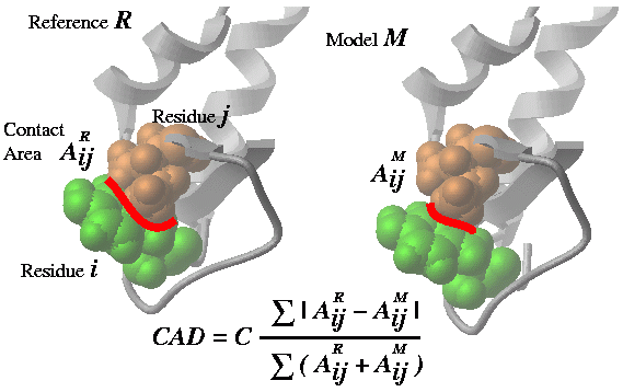
 Cad ( rs_A1 [ rs_A2]  rs_B1 [ rs_B2] [ distance | alignment ] ) 

• by a single selection rs_A1 : all pairs between selected residues (is equivalent to rs_A1 rs_A1 )
• by two residue selections rs_A1 rs_A2: cross pairs between two sets of selected residues (e.g. the contacts between two subunits)

• distance option allows one to compare approximations of the inter-residue contact areas by the Ca and Cbeta positions. This allows one to calculated deformations between two homologous proteins which is not possible in the default mode in which two chemically identical molecules are compared. The residue pairs in two homologs are equivalenced according to the alignments linked to the molecules. Residues deleted in a homologue are considered to have zero contact.
• alignment option is described in Marsden, Abagyan, 2004, Bioinformatics, v20, 2333-2344.

# Ab initio structure prediction, Overall models by homology  
   read pdb "cnf1"   # one conformation of a protein  
   read pdb "cnf2"   # another conformation of the same protein 
   show 1.8*Cad(a_1. a_2.)   # CAD=0. - identical; =100. different 
   show 1.8*Cad(a_1.1 a_2.1) # CAD between the 1st molecules (domains) 
   show 1.8*Cad(a_1.1/2:10 a_2.1/2:10) # CAD in a window 
   PLOT.rainbowStyle = 2 
   plot area grid M_out comment=String(Sequence(a_1,2.1)) link display 
 
# Loop prediction: 0% - identical; ~100% totally different 
#    CAD for loop 10:20 and its interactions with the environment 
   show 1.8*Cad(a_1.1/10:20 a_1.1/* a_2.1/10:20 a_2.1/*)   
#    CAD for loop 10:20 itself 
   show 1.8*Cad(a_1.1/10:20 a_1.1/10:20 a_2.1/10:20 a_2.1/10:20)   
 
# Evaluation of docking solutions: 0% - identical; 100% totally different 
   read pdb "expr"   # one conformation of a complex  
   read pdb "pred"   # another conformation of the same complex 
   show Cad(a_1.1 a_1.2 a_2.1 a_2.2)  # CAD between two docking solutions  
# 
# ANOTHER EXAMPLE: the most changed contacts  
   read object "crn" 
   copy a_ "crn2" 
   randomize v_ 5. 
   Cad(a_1. a_2.) 
   show s_out 
   read column group input= s_out name="cont" 
   sort cont.1 
   show cont 
# the table looks like this (the diffs can be both + and -): 
#>T cont 
#>-1-----------2-----------3---------- 
   -39.        a_crn.m/38  a_crn.m/1 
   -36.4       a_crn.m/46  a_crn.m/4 
   -32.1       a_crn.m/46  a_crn.m/5 
   -29.8       a_crn.m/30  a_crn.m/9 
   -25.2       a_crn.m/37  a_crn.m/1 
... 
   42.5        a_crn.m/43  a_crn.m/5 
   45.1        a_crn.m/44  a_crn.m/6 
   45.2        a_crn.m/43  a_crn.m/6 
   55.3        a_crn.m/46  a_crn.m/7 
   56.         a_crn.m/45  a_crn.m/7

 Cad ( rs_A1 [ rs_A2]  rs_B1 [ rs_B2] alignment  ) 

 Ceil ( r_real [ r_base] ) 

 Ceil ( R_real [ r_base] ) 

 Cell ( {  os |  m_map } ) 

 Charge ( { os | ms | rs | as } [ formal | mmff ]  ) 

• formal : return formal charges
• mmff : return formal charges calculated according to mmff atom types and rules. Note: do not confuse this option with a function to return the mmff charges.

build string "ala his glu lys arg asp" 
 show Charge(a_1)      # charge per molecule 
 show Charge( a_1/* )  # charge per residue 
 show Charge( a_1//* ) # charge per atom  
 
 avC=Charge(a_/5)         # total electric charge of 15th residue  
 avC=Sum(Charge(a_/5/*))  # another way to calculate it 
 show Charge(a_//o*)      # array of oxygen charges  
 
# to return mmff charges: 
 set type mmff 
 set charge mmff 
 Charge( a_//* ) 
 
# to return total charges per molecular object: 
 read mol s_icmhome+"ex_mol.mol" 
 set type mmff 
 set charge mmff 
 Charge( a_*. )

Converting 3D objects to chemical arrays.

 Chemical( ms|os [exact] [hydrogen] [unique] [pharmacophore] [stack] )

returns an array of chemicals from a molecular selection of 3D molecular objects, e.g. a_H for hetero-molecules By default the selected molecules will be converted to 2D graphs. However with the exact option the original 3D coordinates will be retained in the elements of the chemical array. If you want to preserve explicitly drawn hydrogens hydrogen option should be used. Note that the number of chemicals in the array will be determined by the selection level. At the object level multiple molecules of the same object will be merged into one array element. With unique option duplicates will be excluded from the result. If 3D object has an embedded conformation stack you can use stack option to preserve it in the result chemical object

Example:

read pdb "1ch8"
group table t_2D Chemical(a_H)   # convert to 2D chemical table 
group table t_3D Chemical(a_H exact)  # make 3D chemical table without hydrogens
group table t_3D_hyd Chemical(a_H exact hydrogen) # make 3D chemical table, keep hydrogens

With pharmacophore option the function generates pharmacophore points for the input selection.

Example:

read object s_icmhome + "biotin.ob" name="biotin"
read mol input = String(  Chemical(a_ pharmacophore )) name="biotin_ph4"
display xstick 
display wire a_biotin.

To display supported pharmacophore types and use show pharmacophore type command

Converting smiles to chemical arrays:

 Chemical( S_smiles|s_smiles )

returns an array of chemicals from a string arrays of smiles.

Example:

add column t Chemical({"N[C@@](F)(C)C(=O)O", "C[C@H]1CCCCO1"})

Converting InChI to chemical arrays:

 Chemical( S_InChI|s_InChI )

See also: chemical functions

Generating combinatorial compounds from a Markush structure and R-group arrays.

 Chemical( scaffold I_RgroupNumArray  enumerate ) → returns one chemical

The I_RgroupNumArray is an array of as many elements as there are different R groups in the scaffold.E.g. if there is R1 R2 R3 than this parameter can be {10,21,8}. The numbers refer to the R-group arrays linked to the scaffold.E.g.

group table scfld Chemical("C(=CC(=C(C1)[R2])[R1])C=1") "mol"
link group scfld.mol 1 Chemical({"N","O","S"})
link group scfld.mol 2 Chemical({"[Cl]", "[C*](=O)O"})

Nof( scfld.mol library ) # returns the total number of molecules in that combinatorial library
Nof( scfld.mol group )   # returns an array of sizes of each linked array in R1 R2.. order.

Chemical( scfld.mol {1 1} enumerate )
Chemical( scfld.mol {1 2} enumerate )
Chemical( scfld.mol {2 2} enumerate )

 Chemical( enumerate scaffold [simple] R1 R2 ... ) → returns enumeration result

The same as above but does not require explicit linkage with link group command.

Example:

Chemical( enumerate  Chemical("C(=CC(=C(C1)[R2])[R1])C=1") Chemical({"N","O","S"}) Chemical({"[Cl]", "[C*](=O)O"}) )

simple mode is similar to enumerate library and requires that size of R-group arrays be the same.

Example:

Chemical( enumerate  Chemical("C(=CC(=C(C1)[R2])[R1])C=1") simple Chemical({"N","O"}) Chemical({"[Cl]", "[C*](=O)O"}) )

See also: linking scaffold to R-group arrays and the Nof

[ Collection ]

 Cluster( I_NxM_NearestNeighb i_M_totalNofNearNeighbors i_minNofCommonNeighbors ) → I_N_clusterNumbers

 Cluster( M_NxNdist r_maxDist ) → I_N_clusterNumbers 

# let us make a distance matrix D 
# we will cook it from 5 vectors {0. 0. 0.} 
 m=Matrix(5,3)  # initialize 5 vectors 
 m[2,1:3]={1. 0. 0.}   # v2 
 m[3,1:3]={1. 1. 0.}   # v3 
 m[4,1:3]={1. 1. 1.}   # v4 
 m[5,1:3]={1. 0.1 0.1} # v5 close to v2 
 
 D = Distance( m )  # 5x5 distance matrix created 
 
 Cluster( D , 0.2 ) # v2 and v5 are assigned to cluster 1 
 Cluster( D , 0.1 ) # radius too small. All items are singlets 
 Cluster( D , 2.  ) # radius too large. All items are in cluster 1

The function to create a collection object

 Collection()

 Collection( s_json_string )

 Collection( s_url_encoded_string )

 Collection( web )

 Collection( S_uniq_names_n S_values_n )  

 Collection( table_row )

 Collection( table {column|header|all} )

 Collection( table|tab_column format )

add column t {1 2 3} {1 2 3}
add column t function= "A+B"
set format t.A "<i>%1</i>"
show format t 
c = Collection(t.A format )  # modify c
set format t.B c

[ Color from gradient | Color image | Color protein ]

• : Color( [ball|cpk|label|skin|surface|wire|ribbon|label] ) => M_Nx3_rgb
• : Color( background ) =>
• : Color( ) => M_Nx3_rgb
• : Color( [] ) => S_system_color_names_or_hex
• : Color( ) => S_n_colorNames from _red to _black
• : Color( [ ] ) => R_3_rgb|M_Nx3_rgb # interpolation
• : Color( protein ) =>
• : Color( [name] ) =>
• : Color( background ) =>
• : Color( [ []] ) =>

 Color ( as_n ball|cpk|label|skin|surface|wire ) → M_nx3_rgb

 Color ( g_grob )  → M_nx3_rgb

build string "se his" 
 display xstick 
 make grob image name="g_" 
 display g_ only smooth 
 M_clr = Color( g_ ) 
 for i=1,20    # shineStyle = "color" makes it disappear completely 
   color g_ (1.-i/20.)*M_clr 
 endfor 
 color g_ M_clr

 Color( M_rgb [name] )  → S_colorHex_or_Names

- returns sarray of color names in hex code, or, with option name , ICM colors approximating the rgb values in the matrix. The ICM color names and definitions are taken from the icm.clr file. Example:

m = Matrix(3)
Color(m ) # returns {"#ff0000","#00ff00","#0000ff"}
Color(m name) # returns icm approximations {"red","lime","midnightblue"}

 Color( system ) 

- returns sarray of system color names.

 Color( system i_numColor ) 

- returns a name of a system color by number.

Example:

N = Nof( Color( system ))
for i=1,10
  print Color( system Random(N) )   # randomly pick one color
endfor

 Color( background ) 

 Color( r_value s_gradient [ r_from r_to ] ) → R_3rgb

 Color( R_N_values s_gradient [ r_from r_to ] )

Note that these colors are from the permanent part of the spectrum and are only approximately equal to transient colors resulting from the color-by-rainbow-and-value command like

GRAPHICS.NtoCRainbow = "white/lightpink/red/darkred"
R = Bfactor(a_/* ) 
color a_/* R//0.//100.   # uses a perfect rainbow at a transient part of the spectrum
Color( R "white/lightpink/red/darkred" 0. 100. ) # projects those colors to the 'named' part of the spectrum

Examples:

s = "red/lime/blue"
Color( 0.  s 0. 1. ) 
Color( 0.5 s 0. 1. )
Color( 1.0 s 0. 1. )
Color( 0.1 s 0. 1. )
Color( 0.8 s 0. 1. )
Color( {0.1 0.8} s 0. 1. )
Color( {1. 8.} s 0. 10. )

Color( 0.1 "red/lime/blue,0:1" )
Color( {0.1 0.8} "red/lime/blue,0:1" )
Color( {1. 8.} "red/lime/blue,0:10" )

 Color( imageArray background )

returns sarray with background colors of the images in imageArray_.The color of the top left pixel of the image is returned as the background color currently.

See also: Image, image parray

 Color( S|s_aa protein ) → S|s_aaHexColors

Some tables may contain an amino acid (along with its position) in its cell, e.g. one may record amino acids around the binding site:

add column t "D12"//"E13"//"K14" "D"//"A"//"L"
show Color(t.A protein )     # returns sarray of colors for each value
show Color(t.A[1] protein )  # returns string color, eg #AAFFFF for "D12"  
set format t.A color='Icm::Color(A protein)'  # will color cells in the table.

See also: set format

 Consensus ( ali ) → s_consensus

 Consensus ( ali { i_seq | seq } ) 

read alignment "sx"  # load alignment  
 read pdb "x"         # structure  
 display ribbon 
        # multiply rs_ by a mask like "  A C   N  .." 
 cnrv = a_/A & Replace(Consensus(sx cd59),"[.^~#]"," ")  
 display cnrv red  
 display residue label cnrv

 Consensus ( ms|rs ) 

surface accessible areas projected on the selected residues via linked sequence and alignment.

making a table with the contour lines of a 2D function represented by a matrix for display in the plot command.

 Contour( M  [r_step|i_numContours [fmin,fmax]] [R_Xs|R_Ys] ) → T_contourData (X,Y,conn,Z)

Example (UNFINISHED):

M = 10.*Smooth(Smooth(Smooth(Matrix(100))))
tt = Contour(M,10,0.,5.)
delete tt.Z == 0.
sort tt.Z
add column tt "_black line 0.5" name="mark" 
plot tt.X tt.Y tt.mark "/tmp/tmp.eps" append

 Corr ( R_X, R_Y ) → r_correlation

Note: this function returns R , not R² . Taking it to the 2nd power can be a humbling experience.
Examples:

r=Corr(a,b)                 # two vectors a and b  
 if (Abs(r_out) < 0.3) print "it is actually as good as no correlation"

 Cos ( { r_Angle | i_Angle } ) 

 Cos ( rarray ) 

show Cos(60.)                           # returns 0.5  
 show Cos(60)                            # the same  
 
 rho={3.2 1.4 2.3}                       # structure factors  
 phi={60. 30. 180.}                      # phases  
 show rho phi rho*Cos(phi) rho*Sin(phi)  # show in columns rho, phi,  
                                         # Re, Im

 Cosh ( { r_Angle | i_Angle } ) 

 Cosh ( rarray ) 

show Cosh(1.)                           # 1.543081  
 show Cosh(1)                            # the same  
 
 show Cosh({-1., 0., 1.})                # returns {1.543081, 1., 1.543081}

•  Count( i_n ) → I_1,2,3,..n 

•  Count( i_from i_to [i_step=1] ) → I_from,...,to 

•  Count( I|R|S_array ) → I_1,..,n

•  Count( I|R|S unique|identity|number) → I # 111222233 or 123123412 or 333444422

Detailed descriptions:


 Count ( [ i_Min, ] i_Max ) 

- returns iarray of numbers growing from i_Min to i_Max. The default value of i_Min is 1.
Examples:

show Count(-2,1)         # returns {-2,-1,0,1}  
 show Count(4)            # returns {1,2,3,4}

See also the Iarray( ).


 Count ( array ) 


- returns iarray of numbers growing from 1 to the number of elements in the array.

 Count ( I|R|S_array unique | identity )  → I

returns an integer array with integer id for sequentially identical values. Example:

group table t {"d","d","d","bb","bb","a","a","a"} 
add column t Count(t.A unique ) Count(t.A identity ) name={ "unique","identity" }
show t
 #>T t
 #>-A-----------unique------identity---
    d           1           1          
    d           1           2          
    d           1           3          
    bb          2           1          
    bb          2           2          
    a           3           1          
    a           3           2          
    a           3           3

---

CubicRoot

 CubicRoot( r ) → r_cubic_root

 CubicRoot( r [ r_im ] ) → R6_3re+3im

Example:

CubicRoot(27. )
  3.
CubicRoot(27. 0.) 
 #>R 
   3.
   -1.5
   -1.5
   0.
   -2.598076
   2.598076

See also: SolveCubic, Sqrt


Date

Summary:




 Date( ) → e_1currentDate

 Date ( filename modify ) → e_dateOfLastFileModification

 Date( n ) → e_arrayOf_n_currentDates

returns an date array of current system date and time. It may be used as a column in a table.

Example:

print "Today is :" Date()
add column t Count(10) Date(10) 
t.B[1] = Date()   # today
t.B[2] = Date()-1 # yesterday
t.B[3] = Date()+1 # tomorrow

 Date ( version ) → e_dateOfCompilation

 Date ( os ) → e_pdbDates

returns the date of the pdb file creation in an date array format. The date read from the HEADER record of a pdb file and is stored with the object.

Example:

read pdb "1crn"
if Date(a_) > Date("1980","%Y") print "released after 1980"

 Date ( {s_date_string|S_dates} [ s_format_to_parse_date_string ] ) 

converts string or sarray to dates using s_format or default TOOLS.dateFormat and always returns a parray of dates. If the first argument is a string, it will have one element in the array.

Example:

String( Date( "12 Oct 2002", "%d %b %Y" ) "%Y-%m-%d" )

The allowed format specifications are the following:

format	description
%a or %A	The weekday name according to the current locale, in abbreviated form or the full name.
%b or %B	The month name according to the current locale, in abbreviated form or the full name.
%c	The date and time representation for the current locale.
%C	The century number (0-99).
%d or %e	The day of month (1-31).
%D	Equivalent to %m/%d/%y. (This is the American style date, very confusing to non-Americans, especially since %d/%m/%y is widely used in Europe.)
%H	The hour (0-23).
%I	The hour on a 12-hour clock (1-12).
%j	The day number in the year (1-366).
%m	The month number (1-12).
%M	The minute (0-59).
%n	Arbitrary whitespace.
%p	The locale’s equivalent of AM or PM. (Note: there may be none.)
%r	The 12-hour clock time (using the locale’s AM or PM). (%I:%M:%S %p)
%R	Equivalent to %H:%M.
%S	The second (0-60; 60 may occur for leap seconds; earlier also 61 was allowed).
%t	Arbitrary whitespace.
%T	Equivalent to %H:%M:%S.
%U	The week number with Sunday the first day of the week (0-53). The first Sunday of January is the first day of week 1.
%w	The weekday number (0-6) with Sunday = 0.
%W	The week number with Monday the first day of the week (0-53). The first Monday of January is the first day of week 1.
%x	The date, using the locale’s date format.
%X	The time, using the locale’s time format.
%y	The year within century (0-99). When a century is not otherwise specified, values in the range 69-99 refer to years in the twentieth century (1969-1999); values in the range 00-68 refer to years in the twenty-first century (2000-2068).
%Y	The year, including century (for example, 1991).

Example:

String( Date() "%b %d %Y %I:%M%p" )  # Current date and time in American style
String( Date() "%d/%b/%Y %H:%M" )    # European style

---

Deletion

 Deletion ( rs_Fragment, ali_Alignment [, seq_fromAli ] [, i_addFlanks ] [{"all"|"nter"|"cter"|"loop"}] )  


- returns the residue selection which flanks deletion points from the viewpoint of other sequences in the ali_Alignment. If argument seq_fromAli is given (it must be the name of a sequence from the alignment), all the other sequences in the alignment will be ignored and only the pairwise sub-alignment of rs_Fragment and seq_fromAli will be considered. The alignment must be linked to the object. With this function (see also Insertion function) one can easily and quickly visualize and/or extract all indels in the three-dimensional structure. The default i_addFlanks parameter is 1. String options:
• "all" (default: no string option) select deletions of all types
• "nter" select only N-terminal fragments
• "cter" select only C-terminal fragments
• "loop" select only the internal zones of deleted loops

See example coming with the Insertion( ) function description.

---




Descriptor (topological and numericals)

 Descriptor ( chemArray number )

- returns table of various numerical descriptors of the following categories:

# https://www.epa.gov/sites/production/files/2015-05/documents/moleculardescriptorsguide-v102.pdf

• Atom counts
  • a_count - total atom count
  • a_heavy - heavy atom count
  • a_aro - aromatic atom count
  • HB_a - hydrogen bond acceptor count
  • HB_don - hydrogen bond donor count
  • Individual atom counts
    • a_nH a_nC a_nN a_nO a_nF a_nP a_nS a_nCl a_nBr
• Bond counts
  • b_count - total number of bonds
  • b_heavy - number of bonds between heavy atoms
  • b_rotN - number of non-ring bonds
  • b_rotR - fraction of non-ring bonds
  • b_1rotN - number of single non-ring bonds
  • b_1rotR - fraction of single non-ring bonds
  • b_ar - number of aromatic bonds
  • b_single - number of single bonds
  • b_double - number of double bonds
  • b_triple - number of triple bonds
  • b_rot - number of aromatic bonds
• Topological Descriptors ([Hall 1991] and [Hall 1997])
  • Definitions
    • n[i] : atomic number of atom i
    • d[i] : number of heavy connections for atom i
    • v[i] : nV[i] - nH[i] for atoms with atomic number <= 10, (nV[i] - nH[i]) / (n[i] - nV[i] - 1) for atoms with atomic number > 10
    • P[i] : number of paths of bond length i in hydrogen suppressed molecule
    • N : number of non-hydrogen atoms
    • R[i] : van der Waals radius of atom i
    • Rc : van der Waals radius of carbon atom
    • α : 1 - Sum( R[i] / Rc )
    • Na : N + α
    • Pa[i] : P[i] + α
  • Chi Connectivity Indices
    • t_chi0 : Atomic connectivity index order 0. Sum(1/sqrt(d[i]))
    • t_chi0_C : Carbon connectivity index order 0. (Same as above calculated for carbon atoms)
    • t_chi1 : Atomic connectivity index order 1. Sum(1/sqrt(d[i]*d[j])) for all bonds between heavy atoms i and j.
    • t_chi1_C : Carbon connectivity index order 1. (Same as above calculated for carbon atoms)
    • t_chi0v : Atomic valence connectivity index order 0. Sum(1/sqrt(v[i]))
    • t_chi0v_C : Carbon valence connectivity index order 0. (Same as above calculated for carbon atoms)
    • t_chi1v : Atomic valence connectivity index order 1. Sum(1/sqrt(v[i]*v[j])) for all bonds between heavy atoms i and j.
    • t_chi1v_C : Atomic valence connectivity index order 1. (Same as above calculated for carbon atoms)
  • Kappa Shape Indices
    • k1 : First kappa shape index: N(N-1)^2 / P[1]^2
    • k2 : Second kappa shape index: (N-1)(N-2)^2 / P[2]^2
    • k3 : Third kappa shape index: (N-1)(N-3)^2 / P[3]^3 for odd N, (N-3)(N-2)^2 / P[3]^2 for even N
    • k1a : First kappa shape index α: Na(Na-1)^2 / Pa[1]^2
    • k2a : Second kappa shape index: (Na-1)(Na-2)^2 / Pa[2]^2
    • k3a : Third kappa shape index: (Na-1)(Na-3)^2 / Pa[3]^3 for odd N, (Na-3)(Na-2)^2 / Pa[3]^2 for even N
  • zagreb : Sum(d[i]*d[i]) for all non-hydrogen atoms
  • weiner : Sum(D(i,j)) for all non-hydrogen atom pairs i,~~j. D(i,j) - topological distance between atoms i and j.
  • maxdist : Max(D(i,j)) for all atom pairs i,~~j. D(i,j) - topological distance between atoms i and j.

Example:

read table s_icmhome + "celebrex50.sdf" name="t"
add column t Descriptor( t.mol number )

Descriptor

 Descriptor ( chemArray )

 Descriptor ( chemArray collection_of_Fingerprint_Parameters [info] ) 

- returns vector of binary fingerprints, default or custom, calculated for each chemical.

The collection_of_Fingerprint_Parameters argument is a collection which defines parameters for fingerprint generation and consists of the following members:

• ATMAP: string with comma separate atom properties descriptions. Example: cd,h
• BOMAP: string with comma separate bond properties description. Example: bt,r
• SIZE : result vector size
• LEN : maximum fragment/chain length
• TYPE : fingerprint type: "linear","triplets","ecfp"
• BINARY: yes/no (no - counted fingerprint mode)
• ECFPITER: (ecfp only) number of iterations. 1 - ECFP2, 2 - ECFP3, 3 - ECFP4, etc...

Examples:

# export default binary fingerprints
  write sarray Sarray(Descriptor(t.mol)) name="fp.txt"

# linear counted fingerprint, SIZE=1024, max chain length=5 
Descriptor( t.mol, Collection("ATMAP" "cd,h" "SIZE" 1024 "BOMAP" "bt,r" "LEN" 5 "TYPE" "linear", "BINARY", no) )
# ecfp4 fingerprint
Descriptor( t.mol, Collection("ATMAP" "cd,h" "SIZE" 2048 "BOMAP" "bt" "LEN" 999 "TYPE" "ecfp", "ECFPITER" 3, "BINARY", no)  )

Example in which fingerprints returned by the function are directly used in distance calculation:

add column t Chemical({"CCN","CCCN"})
mod = Collection()
mod['FP'] = Descriptor( t.mol )
Distance(mod['FP'], Descriptor(Chemical("C(=O)CCN")))

 Descriptor ( chemArray predModel ) 

- returns vector of rarrays with chemical descriptors calculated for each chemical. each rarray consists of chemical fingerprint part and values for columns with formula used in the predModel.

This information can be used for further analysis or exported outside ICM.

Example:

# assumes that 'clogPpred' is a prediction model 
 tt = Table( Transpose( Matrix( Descriptor( Chemical("CCC"), clogPpred ) ) ))
 add column tt Name( clogPpred column )
 sort reverse tt.A

To find the description of the each particular position in the rarray Name function can be used.

Example:

rr = Descriptor( Chemical("CCC") myModel )[1]
na = Name( myModel column )
for i=1,Nof(rr)
  if (rr[i] != 0) print rr[i], na[i]
endfor

See also: Name( predModel, column .

Det

determinant function.


 Det ( matrix ) 


- returns a real determinant of specified square matrix.
Examples:

a=Rot({0. 0. 1.}, 30.)     # Z-rotation matrix by 30 degrees  
 print Det(a)               # naturally, it is equal to 1.

---




Disgeo

Solves the so called "DIStance GEOmetry" problem (finding coordinates from a distance set). This function can be used to visualize in two or three dimensions a distribution of homologous sequences:

group sequence se1 se2 se2 se4 mySeqs 
 align mySeqs 
 distMatr=Distances(mySeqs)


or any objects between which one can somehow define pairwise distances. Since principal coordinates are sorted according to their contribution to the distances and we can hardly visualize distributions in more than three dimensions, the first two or three coordinates give the best representation of how the points are spread in n-1 dimensions. Another application is restoring atomic coordinates from pairwise distances taken from NMR experiments.


 Disgeo ( matrix ) 


- returns matrix [1:n,1:n] where the each row consists of n-1 coordinates of point [i] sorted according to the eigenvalue (hence, their importance). The first two columns, therefore, contain the two most significant coordinates (say X and Y) for each of n points. The last number in each row is the eigenvalue [i]. If distances are Euclidean, all the eigenvalues are positive or equal to zero. The eigenvalue represents the "principal coordinate" or "dimension" and the actual value is a fraction of data variation due to the this particular dimension. Negative eigenvalues represent "non-Euclidean error" in the initial distances.
• R_out returns four numbers: total negative eigen values, and the first 3 largest positive eigenvalues. All scaled to 100%.

Example:

read sequences s_icmhome+"zincFing"   # read sequences from the file, 
 list sequences              # see them, then ...  
 group sequence alZnFing     # group them, then ...  
 align alZnFing              # align them, then ...  
 a=Distance(alZnFing)        # a matrix of pairwise distances  
 n=Nof(a)                    # number of points  
 b=Disgeo(a)                 # calculate principal components  
 corMat=b[1:n,1:n-1]         # coordinate matrix [n,n-1] of n points  
 eigenV=b[1:n,n]             # vector with n sorted eigenvalues  
 xplot= corMat[1:n,1] 
 yplot= corMat[1:n,2] 
 plot xplot yplot CIRCLE display # call plot a 2D distribution

---




Distance

[ Distance iarray | Distance rarray | Distance ~~as_ | Distance ~~as_ rarray | Distance matrix | Distance hierarchical | Distance Tanimoto | Distance chemset | Distance 2 matrices | Distance tether | Distance Dayhoff | Distance in alignment | Distance 2 alignments | Distance tree | Distance chemical ]

generic distance function. Calculates distances between two ICM-shell objects, bit-strings or molecular objects, or extracts distances from complex ICM-shell objects.

 Distance( II | RR | as as | seq seq ) → r_dist

 Distance( S|s, s) → R|r

 Distance( ali ali [exact] ) → r

 Distance( S S [simple]) → M

 Distance( Sn_hier_codes Sm_hier_codes tree [ s_delimeter ]) → M_nm_0to1

 Distance( Mnk ) → Mnn_cart_dist_between_row-vectors

 Distance( Mnk Mmk ) → Mnm

 Distance( M_xyz|as M_xyz|as r_dist ) → l_yes_if_closer_than_dist

 Distance( seq seq [identity|evolution|new|fast|number|reverse] )

 Distance( seq seq nucleotide [len] )

 Distance( seqArr[n]> ) → <M_nn

 Distance( ali seq [string] ) → R_n_seq_in_ali

 Distance( seqArr[n]> <seq ) → R_n

 Distance( seqArr[n]> <seqArr[m]> ) → <M_nm

 Distance( as [r_default=-1.] ) → R_tether_lengths_or_def

 Distance( as_n as_m ) → d_between_centers_of_mass

 Distance( as_n as_m all ) → R_nm

 Distance( as_n as_n rarray ) → R_n # aligned arrays, same n 

 Distance( ali [0] ) → M_interSeqDist

 Distance( X_n [X_m] [pharmacophore|sstructure] ) → M_nxm_chemical_Tanimoto_distances

 Distance( X_n X_m [[R_Wn R_Wm] r_maxdist (0.4) [r_steepness(6.)]] set ) → r_set1_2_distance

 Distance( bitvecArr[n]> <bitvecArr[m]> ) → <M_nm #tanimoto, see Descriptor function

 Distance( I_keys1 I_keys2 i_nBits|R_nbitWeights [simple] ) → M : Tanimoto|weighted 

 Distance( tree [i_at=1] split ) → r_splitLevel

 Distance( tree all|modify ) → R_splitLevels|splitLevelTStats

 Distance( g wire|grid [i_maxDist(1000000)>] ) → <M_shortestPaths

 Distance( d_0to1|M evolution ) → d|M_Dayhoff_correction_applied

See detailed descriptions below.


Distance between iarrays

 Distance ( iarray1,  iarray2 ) 


- returns the real sqrt of sum of (I1_i -I2_i )² .


Distance between vectors

 Distance ( R_X,  R_Y ) 

- returns the real Cartesian distance between two vectors of the same length. D = Sum( ( X_i - Y_i )² )


Distance ~~as_

 Distance ( as_1, as_2 [ all ] ) 

- returns the real distance in Angstroms between centers of mass of the two specified selections. The interactive usage of this function: Option all will return an array of all cross distances between the selections. The selected virtual atoms will be skipped if the selection level residue, molecule or object. Othewise, if you explicitly select virtual atoms, they will be included, e.g.

build string "ala" # contains 2 virtual atoms at N terminus
 build string "his" # also contains 2 virtual atoms at N terminus
 Distance( a_1. a_2. all ) # no virtual atom distances
 Distance( a_1.// a_2.// all ) # selected virtual atoms are included

 Distance( a_1. a_2. ) # a single distance between centers of mass




Distance ~~as_ rarray

 Distance ( as_1 ,  as_2,  rarray ) 

- returns the rarray of distances in Angstroms between the two specified selections containing the same number of atoms (1-1, 2-2, 3-3, ...).

See also: Distance ( as1 as2 all )


Distance matrix

 Distance ( M_coor ) 

- returns the square matrix of distances between the rows of the input matrix M_coor. Each row contains m coordinates (3 in 3D space). For example: Distance(Xyz(a_//ca)) returns a square matrix of Ca-Ca distances.

Distance between string arrays of hierarchical labels

 Distance( Sn_hier_codes Sm_hier_codes tree [s_delimeter]) → M_nm 

compares two arrays of hierarchical labels like this: "clan.family.subfamily.." The labels can be delimiter separated, or just strings of the same length where one positions is just one character (the default). Returns a distance matrix normalized to [0:1] range.

Here are examples of classification codes that can be used:

• EC numbers, enzymes: eg Distance({"6.2.1.11"},{"6.2.1.25"}, tree, ".")
• ATC drug codes, eg Distance({"C-03-C-C-01"},{"L-01-A-B-03"}, tree, "-") , use Replace to insert dashes between sections
• AHFS drug codes, eg Distance({"08:18.32"},{"08:16.00","92:00.00"}, tree, ":.")
• ...

Examples:

add column t {"Cocaine","Betaxolol"} {"52:16.00","52:92.00"}
show Distance(t.B t.B tree ":.")
 
add column tt {"Cocaine","Betaxolol"} {"AB2","ABc"}
show Distance(tt.B tt.B tree ) # use each character as level

These distance matrices can be used for making 2D and 3D graphs, or to plot clustering trees of tables containint suitable label columns, eg see ds3D make tree object .

Tanimoto distance between two arrays of bit-strings

 Distance( X_chem_n X_chem_m ) → M_nxm_distances 

 Distance( I_keys1 I_keys2 nBits | R_nBitWeights [simple] ) → M_distances 


- returns the matrix of Tanimoto distances between two arrays of bit-strings. Each array of N-strings is represented by an iarray I_keys of N*( nBits/32 ) elements (e.g. if nBits is 32 , each integer represents 1 bit-string, if nBits i 64, I_keys1 has two integers for each bit string, etc.). The returned matrix dimensions are N1 x N2 . The distance is defined as 1. - similarity , where The Tanimoto similarity between bitstrings is defined as follows: The number of the on-bits in-common between two strings divided by the number of the on-bits in either bit-string.
You can provide a relative weight for each bit in a bit-string as a rarray R_weights. In this case the weighted Tanimoto distance is calculated as follows:

distWeighted = 1. - Sum( Wi_of_common_On_Bits ) / Sum( Wi_of_On_Bits )


With option simple the similarity calculation is modified so that the number of bits in common is divided by the number of bits in the second bit-string. For example:

Distance({3} {1} 32 simple ) # returns 0. 
Distance({1} {3} 32 simple ) # returns 0.5


Example:

Distance({1 2 3},{1 2 3},32) 
 #>M 
 0. 1. 0.5 
 1. 0. 0.5 
 0.5 0.5 0.

The diagonal distances are 0; no bits are share between 1 (100..) and 2 (010..) (distance=1.) and one of two bits is shared between 1 (100..) and 3 (110..).
Instead of the number of bits, one can provide the relative weights for each bit. The dimension of the bit-weight array then becomes the size of the bit-string. The weighted Tanimoto is calculated.

See also:

• Distance(X, X, .., set) to calculate a single distance between two chemical sets
• Score(X, X, .., set)
• Iarray-bits-to-integers{ Iarray({1 0 0 1 1 0 ..} key ) } to generate compressed integer bit vectors

Similarity score between two sets of ligands

 Distance( X_n X_m [[R_Wn R_Wm] r_minScore (0.3) [r_steepness(6.)]] set ) → r_distance [0:1]

retuns a real effective distance between two chemical sets. It is equal to 1 - r_similarity defined by function Score(X1,X2,..set) See also:

• Score(X, X, .., set)



Distance matrix between two sets of coordinates

 Distance ( M_coor1  M_coor2  ) 

- returns the matrix of distances between the rows of the two input matrices. Each matrix row may contain any number of coordinates coordinates (3 in 3D space).
For example: Distance(Xyz(a_/1:5/ca) Xyz(a_/10:12/ca) returns a 5 by 3 matrix of distances between Ca-s of the two fragments.

  Distance( M_xyz1|as1 M_xyz2|as2 r_dist ) → l_yes_if_closer_than_dist

This function returns a logical yes if any two points or atoms in two sets of coordinates or selections are closer than the threshold.


  if Distance   ( as1 as2 r_dist ) then ...

is a more efficient version of this condition:

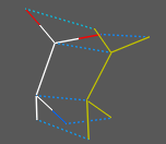
  if Nof( Sphere( as1 as2 r_dist )) > 0 




Distance tether

 Distance ( as [ r_defaultLength=-1.] ) 


- returns the real array of lengths of tethers for each selected atom or the default value ( -1. ). The default value can be set to any value. Tethers are assumed to be already set, see command set tether. Also note, that the expression Distance( as_out ) will give the same results if as_out selection was not changed by another operation; see also special selections.
Example:

read pdb "1crn" convert tether # keeps tethers to the pdb original deviations = Distance( a_//!h*,vt* , 9.9) perResDevs = Group( deviations, a_//!h*,vt* ,"max") # find max.devs per residue display ribbon color ribbon a_/* perResDevs # Another example Distance( a_//T ) # selects only tethered atoms #>R 1.677 1.493 1.386 1.435 1.645 1.570 2.165 1.399




Distance Dayhoff

  Distance( seq1 seq2 [identity|evolution|new|fast|number|reverse] ) → r

  Distance( r_dist_0_to_1|M_dist ) → r|M_Dayhoff_corrected_distances to [0.:10.]

  Distance( seqArr[n] seq ) → R_n

 Distance( d_0to1|M evolution ) → d|M_Dayhoff_correction_applied

- returns the real measure of difference between two aligned sequences. Zero distance means 100% identity. The distance is calculated by the following two steps:

1. d1 = 1.0 - (nResidueIdentities/Min(Length(Seq1), Length(Seq2)) (d1 belongs to [0.,1.] range)
2. if there is no identity option (or the sequence option for a general value to value transformation), the distance is corrected: Distance(Seq1,Seq2) = DayhoffTransformation( d1 )

Transformation practically does not change small distances d1, whereas large distances, especially above 0.9 (10% sequence identity) are increased to take occasional reversals into account. Distances d1 within [0.9,1.0] are transformed to [5.17, 10.] range.

The last function ( Distance( d|M evolution ) allows to apply Dayhoff correction that extends a distance from 0. to 1. to a range 0. to 10. to take into acount the evolutionary time correction (stretching) at larger distances because.

See also: Distance ( ali ) for distance and seq.identity matrices.




Distance between sequences or alignment sequences

  Distance ( alignment ) → M_nxn

  Distance( seqArr_n ) → M_nxn

  Distance( seqArr_n seqArr_m ) → M_nxm

- returns matrix of pairwise sequence-sequence distances in the alignment. These distances are calculated with the fast option as follows

1. for each pair of sequences in multiple alignments calculate sequence identity according to the alignment as:

   1.-(nResidueIdentities)/Min(Length(Seq1), Length(Seq2))

   the resulting number will be between 0. and 1.
2. apply the Dayhoff correction formula that will convert the linear distance to 'evolutionary' distance (kind of evolutionary time needed to arrive at this identity. Where the inifinite time is defined as 10. The resulting distance will be between 0. and 10. and area of 'insignificant linear distances' will be pushed to larger than 1. values. Between two identical sequences D= 0. , while the distance between two 30% different sequences will be around 0.5. The distance goes to an arbitrary number of 10. for completely unrelated sequences.

Example:

read alignment msf s_icmhome+"azurins"            # read azurins.msf  
 NormCoord = Disgeo(Distance(azurins))   # 2D sequence diversity in  
#
# calculate pairwise sequence identities
 read alignment "aln" name="aln"
 n=Nof(aln)
 mids = 100*(Matrix(n,n,1.) - Distance(aln ))  # the pairwise seq. identities
 t = Table( mids, Name(aln), Name(aln) )  # to convert the matrix into pairwise table
 t = Table( mids, index )  # a simpler version with i,j




Distance between two alignments

 Distance ( ali_1  ali_2 [ exact ] ) 

- returns the real distance between two alignments formed by the same sequences.
The distance is defined as a number of non-gap columns identical between two alignments.
Two different normalizations are available:
The default normalization is to the shorter alignment. ( Distance ( ali_1 ali_2 ) ). In this case the number of equivalent pairs is calculated and is divided by the total number of aligned pairs in the shorter alignment. This method detects alignment shifts but does not penalize un-alignment of previously aligned residue pairs. D = (La_min - N_commonPairs)/La_min In the following alignment the residue pairs which are aligned in both alignments are the same, therefore the distance is 0.

show a1   # La1 = 3 
 ABC---XYZ 
 ABCDEF--- 
 show a2   # La2 = 6 
 ABCXYZ 
 ABCDEF 
 Distance(a1,a2)   # a1 is a sub-alignment of a2, distance is 0. 
 0.


exact option: normalization to the number of pairs of the longer alignment. By longer we mean the larger number of aligned pairs regardless of alignment length (the latter includes gaps and ends). D = (La_max - N_commonPairs)/La_max Now in the above example, La_max = 6 , while N_commonPairs = 3, the distance is 0.5 (e.g. the alignments are 50% different).

Distance(a1,a2,exact)  # returns 0.5 for the above a1 and a2


Example showing the influence of gap parameters:

read sequence msf s_icmhome+"azurins.msf"  
 gapOpen =2.2 
 a=Align(Azu2_Metj  Azup_Alcfa)   # the first alignment 
 gapOpen =1.9                     # smaller gap penalty and .. 
 b=Align(Azu2_Metj  Azup_Alcfa)   # the alignment changes 
 show 100*Distance(a b )          # 20% difference 
 show 100*Distance(a b exact )    # 21.7% difference 
 show a b

The distance of the cluster splitting level

 Distance( treeArr i_at separator )

- return the current value of the cluster splitting level set by split command.


Chemical similarity distance

 Distance( chemarray [pharmacophore] )

- return square matrix of chemical distances. The chemical distance is defined as the Tanimoto distance between binary fingerprints Option pharmacophore uses different fingerprints based on ph4-type triplets.

Example:

Distance( Chemical( { "CCC", "CCO"} ) )

 Distance( chemarray1 chemarray2 [pharmacophore] )

- return a MxN matrix where M is number of elements in chemarray1 and N is number of elements in chemarray2 Option pharmacophore uses different fingerprints based on ph4-type triplets.

Example:

Distance( Chemical({ "CCC", "CCO"}) Chemical("CC" ))

Zero distance for non-identical compounds.Sometimes non-identical compounds can give a zero fingerprint distance due to the limitations inherent in finite length fingerprints. To make the distance more representative, one can mix different types of distances, e.g. for two chemical arrays X1 and X2

Mdist = Distance( X1, X2 ) + 0.1*Distance(X1,X2, pharmacophore)

See also: find table find molcart other chemical functions

---

Eigen

eigenvalues/eigenvectors function, eigendecomposition of a square diagonal matrix.


 Eigen ( M  ) → X_eigenVectorColums  and R_out with eigen values


- returns the square matrix ( n x n ) of eigenvector columns of the input symmetric square matrix M_ . All n eigenvalues sorted by their values are stored in the R_out rarray.

Eigen value decomposition is be given by three matrices: X, Matrix(3,R_out) and Power(X,-1)
Example of an eigen-value decomposition:

# create a symmetric real matrix which describes a transformation
read matrix name="A" input="""
2. 0.6 0.5 
0.6 4. 0.3 
0.5 0.3 6. 
"""
 X = Eigen(A)              # calculate eigenvectors... 
 V = R_out                 # and save eigenvalues in rarray V 
 L = Matrix(3,V)           # diagonal matrix with eigen values
# note that now A can be reproduced by this calculation : X*L*X^^-1
 show A,  X*L*Power(X,-1)
# Eigenvectors are X[?,1],  X[?,2], X[?,3]
 show X[?,1]  # 1st eigen-vector

---




Energy

function.


 Energy ( string ) 


- returns the real sum of pre-calculated energy and penalty (i.e. geometrical restraints) terms specified by the string.
Important: this function does NOT calculate the energy, the terms must be calculated beforehand by invoking one of the following commands where energy is calculated at least once: show energy, minimize, ssearch command and montecarlo command.
Note:
• Allowed terms in the string are "vw,14,hb,el,to,af,bb,bs,cn,tz,rs,xr,sf";
• "func" stands for the total of all the terms, both energy and penalty;
• "ener" is only the energy part (i.e. "vw,14,hb,3l,to,af,bb,bs,sf" );
• "pnlt" is only the penalty part (i.e. "cn,tz,rs,xr" ).
• load conf and load frame commands fill out all the energy/penalty terms, which are stored in both stacks and trajectory files (of course the values also depend on a set of free variables). You can get the energy/penalty terms of the loaded conformation without explicitly recalculating them using the Energy function, e.g. Energy("func")



 Energy ( rs [ simple | base | s_energyTerms ] ) 


- in contrast to the previous function this function with an explicit residue selection calculates and returns residue energies in an ICM object. convert the object if is not of the ICM type. The energies are calculated according to the current energy terms , and also depend on the fixation of the object. Note: Use unfix only V_//S,V before the function call for standard fixation.
This function can be used to evaluate normalized residue energies for standard amino-acids to detect local problems in a model.

For normalized energies, use the simple option. The base option just shifts the energy value to the mean energy for this residue type. If the simple or base terms are not used, the current energy terms are preserved. The energies calculated with the simple or base option are calculated with the "vw,14,hb,el,to,en,sf" terms. The terms are temporarily enforced as well as the vwMethod = 2 and vwSoftMaxEnergy values, so that the normalization performed with the simple option is always correct. Do not forget to

build string "ASDF"
unfix only V_//S,V
add column t Name(a_/A full) Energy( a_/A simple )  Energy( a_/A base )
show t


This function will calculate residue energies for all terms and set-ups with the following exceptions:
• electrostatic ( "el" ) term and electroMethod = "boundary element", "MIMEL", or "generalized Born"

The s_energyTerms argument allows one to refine the energy terms dynamically (see example below).
Example:

read pdb "1crn" 
  delete a_W 
  convert 
  set terms "vw,14,hb,el,to,en,sf" 
  group table t Energy( a_/A ) "energy" Label(a_/A ) "res" 
  show t 
  unfix V_//* 
  group table tBondsAngles Energy( a_/A "bs,bb" ) "covalent" Label(a_/A ) "res" 
  show tBondsAngles


See also: the calcEnergyStrain macro.


 Energy ( conf  i_confNumber) 


- returns the table of all the energy components for a given stack conformations.
The table has two arrays:
• sarray of the energy term names ( .hd ) and
• rarray of energy values for each energy term ( .ey ) and



 Energy ({ stack | conf } )  


- returns the rarray of total energies of stack conformations. Useful for comparison of spectra from different simulations.
Examples:

read object s_icmhome+"crn.ob"
 set terms only "vw,14,hb,el,to"  # set energy terms  
 show energy v_//xi*              # calculate energy with only  
                                  # side chain torsions unfixed  
           # energy depends on what variables are fixed since  
           # interactions inside rigid bodies are not calculated,  
           # and rigid body structure depends on variables  
 
 a = Energy("vw,14")      # a is equal to the sum of two terms  
 
 electroMethod="MIMEL"    # MIMEL electrostatics  
 set terms only "el,sf"   # set energy terms  
 show energy 
 print Energy("ener")     # total energy  
 print Energy("sf")       # only the surface part of the solvation energy  
 print Energy("el")       # electrostatic energy  
 print r_out              # electrostatic part of the solvation energy

---

Entropy

 Entropy( R_frequencies ) → r_entropy

 Entropy( R_energies r_RT_energy ) → r_entropy

 Entropy( seq [simple|R_26aa_prob] ) → r_entropy

returns energy calculated as ∑_i p_i Log(p_i) where p_i probabilities are calculated either as normalized R_frequencies or exp( -(E-E_min)/ r_kT_energy ) factors.

If the frequency array contains only one element it is considered as the first probability of an array of two probability that should add up to 1., ie {0.2} is interpreted as {0.2, 0.8}.

The sequence entropy is calculated according to the residue probability from a standard amino acid frequency table. You may substitute it with your own array of 26 numbers. Option simple assumes residue frequencies to be 1/20.

Notes:

• note that the entropy is unit-less generally proportional to the number of comparable high frequency/low_energy states.
• Natural logarith (base e ) is used for the calculation
• for Shannon entropy one needs to multiply the answer by 1./Log(2.) ≃ 1.4427
• if one uses molar energies in kcal/mol , the temperature factor will be RT ≃ 0.6 kcal/mol

Examples:

Entropy({0.5, 0.5})      # 0.693147, two equi-prob. states
Entropy({0.2})           # 0.500402, two states: p=0.2 and p=0.8
Entropy({0.2, 0.2, 0.2})       # 1.09861  three states, 
Entropy({10.2, 0.2, 0.2, 0.2}) # 0.275593 one estates dominates
# below the numbers are interpreted as energies, and 1.4 is a temperature factor.
Entropy({-30., -28., -31., -15.}, 1.4) # 0.848429. ΔEs divided by 1.4, exponentials used to calc probs. 
Entropy({-30., -28., -31., -15.},100.) # 1.38432 at this high temperature 4 states are almost equi-probable.




Error

function indicates that the previous ICM-shell command has completed with error.


 Error 


- returns logical yes if there was an error in a previous command (not necessarily in the last one). After this call the internal error flag is reinstalled to no. The shell error flag can be set to yes with the set error command.

 Error ( string ) 


- returns string with the last error message. It also returns integer code of the last error in your script in i_out . In contrast to the logical Error() function, here the internal error code is not reinstalled to 0, so that you can use it in expressions like if( Error ) print Error(string) .


 Error ( i_error_or_warning_code )  → l 

 Error ( number )  → s 

- returns logical yes if an error or warning with the specified code occurred previously in the script. This call also resets the flag (e.g. Error(415) ). This is convenient to track down certain warnings or errors in scripts (e.g. detecting if 'readpdb{read pdb} found certain problems).
Option number will return a string will previously set error and warning messages.
To clear all bits use the clear error command.

Examples:

read pdb "1mng"  # this file contains strange 28-th residue  
 if (Error) print "These alternative positions will kill me" 
 
 read pdb "1abcd"  # file does not exist 
 read pdb "1mok" 
 clear error

See also: errorAction , s_skipMessages , l_warn, Warning


 Error ( r_x [ reverse ] ) 


- returns real complementary error function of real x : erfc(x)=1.-erf(x)) , defined as
(2/sqrt(pi)) integral{x to infinity} of exp(-t²) dt
or its inverse function if the option reverse is specified. It gives the probability of a normally distributed (with mean 0. and standard deviation 1./Sqrt(2.)) value to be larger than r_x or smaller than -r_x.
Examples:

show 1.-Error(Sqrt(0.5)) # P of being inside +-sigma (about 68%) 
 show Error(2.*Sqrt(0.5)) # P of being outside +- 2 sigma




 Error (  R_x ) 


- returns rarray of erfc(x)=1.-erf(x)) functions for each element of the real array (see above).
Examples:

x=Rarray(1000 0. 5. ) 
 plot display x Error(x ) {0. 5. 1. 1. 0. 1. 0.1 0.2 } 
 plot display x Log(Error(x ),10.) {0. 5. 1. 1.}   
       #NB: can be approximated by a parabola 
       #to deduce the appr. inverse function. 
       #Used for the Seq.ID probabilities.

Error (for SOAP messages)

 Error( soapMessage )

- returns a error string from the SOAP message. (empty string if no error)

This function is used the check the result of calling SOAP method.

See: SOAP services for more details and examples.

---




Exist

[ Exist-pattern | Exist molcart ]

function indicates if an ICM-entity exists or not.


 Exist ( s_fileName [ write | read | directory ] ) 

- returns logical yes if the specified file or directory exists, no otherwise. Options:
• write open for writing
• read open for reading
• directory the provided string is a directory (not file)

 Exist( collection s_fieldname )

Checks if the field exists, e.g.

c = Collection(); c['a']=123
Exist(c,'a')  # yes
Exist(c,'b')  # no

 Exist ( key,  s_keyName ) 

- returns logical yes if the specified keystroke has been previously defined. Examples: Exist(key, "F1" , Exist( key, "Ctrl-B" ) See also: set key command.


 Exist ( object ) 

- returns logical yes if there is at least one molecular object in the shell, no otherwise.


 Exist ( os1 stack ) 

- returns logical yes if there is a built-in object stack , no otherwise.


 Exist ( box ) 

- returns logical yes if the purple box is displayed, no otherwise.


 Exist ( view ) 

- returns logical yes if the GL - graphics window is activated, no otherwise.


 Exist ( gui ) 

- returns logical yes if the GRAPHICS USER INTERFACE menus is activated, no otherwise.

 Exist ( grob display  ) 

- returns logical yes if the grob is displayed.


 Exist( connect ) 

- returns logical yes if the mouse rotations are connected to a graphical object ( grob ) or a molecular object.

 Exist( s_table_name sql table ) 

- returns logical yes if there is an sql table with the specified name exists. It works with the Molcart tables or tables accessed via the Sql function.

 Exist( variable s_varName ) 

- returns yes if the variable exists in the ICM shell, no otherwise. See also Type( ). E.g.

Exist(variable, "aaa")  # returns no
 aaa=234
 Exist(variable, "aaa")  # returns yes

Examples:

if (!Exist("/data/pdb/") then 
   unix mkdir /data/pdb 
 endif 
 
 if(!Exist(key,"Ctrl-B")) set key "Ctrl-B" "l_easyRotate=!l_easyRotate" 
 
 if !Exist(gui)  gui simple

---

 Exist( chemarray pattern )

returns logical yes if at least one of the elements contains SMARTS search attributes, no - otherwise.

Example:

Exist( Chemical("[C&H1,N]") pattern )  # returns yes
Exist( Chemical("CCO") pattern ) # return no

Database information

 Exist( s_dbtable sql table )

- returns logical yes if the specified table exists in the database

See also: molcart

Existenv

function indicating if an UNIX-shell environmental variable exists.


 Existenv ( s_environmentName ) 


- returns logical yes if the specified named environment variable exists.
Example:

if(Existenv("ICMPDB")) s_pdb=Getenv("ICMPDB")

See also: Getenv( ), Putenv( ) .

---




Extension

function.


 Extension ( string [ dot ] ) 


- returns string which would be the extension if the string is a file name. Option dot indicates that the dot is excluded from the extension.


 Extension ( sarray [ dot ] ) 


- returns sarray of extensions. Option dot indicates that the dot is excluded from the extensions.
Examples:

print Extension("aaa.bbb.dd.eee")   # returns ".eee"  
 show Extension({"aa.bb","122.22"} dot)         # returns {"bb","22"} 
 read sarray "filelist"                                     
 if (Extension(filelist[4])==".pdb") read pdb filelist[4]

---




Exp

exponential mathematical function (e^x).


 Exp ( real ) 


- returns the real exponent.


 Exp ( rarray )  


- returns rarray of exponents of rarray components.


 Exp ( matrix  ) 


- returns matrix of exponents of matrix elements.
Examples:

print Exp(deltaE/(Boltzmann*temperature))   # probability  
 print Exp({1. 2.})                          # returns { E, E squared }

---




Field

[ Field user ]

function.


 Field ( s [ s_precedingString]  i_fieldNumber [ s_fieldDelimiter] ) 


- returns the specified field. Parameter s_fieldDelimiter defines the separating characters (space and tabs by default). If the field number is less than zero or more than the actual number of fields in this string, the function returns an empty string.
The s_fieldDelimiter string
Single character delimiter can be specified directly, e.g.

Field("a b c",3," ")  # space 
 Field("a:b:c",3,":")  # colon

Alternative characters can be specified sequentially, e.g.

Field("a%b:c",3,"%:")  # percent OR colon

Multiple occurrence of a delimiting character can be specified by repeating the same character two times, e.g.

Field("a  b   c",3,"  ")    # two==multiple spaces in field delim 
 Field("a%b::::c",3,"%::")   # a single percent or multiple colons

You can combine a single-character delimiters and multiple delimiters in one s_fieldDelimiter string.
More examples:

s=Field("1 ener glu 1.5.",3)    # returns "glu"  
 show Field("aaa:bbb",2,":")     # returns "bbb"  
 show Field("aaa 12\nbbb 13","bbb",1) # returns "13"  
 show Field("aaa 12\nbbb 13 14","bbb",2,"  \n\n") # two spaces and two \n .  
# another example 
 read object s_icmhome+"all" 
       # energies from the object comments, the 1st field after 'vacuum' 
 show Rarray(Field(Namex(a_*.),"vacuum",1))




 Field ( S , [ s_precedingString]  i_fieldNumber [ s_fieldDelimiter] ) 


- returns an string array of fields selected from S_ string array . s_fieldDelimiter is the delimiter. If the field number is less than zero or more than the actual number of fields in this string, an element of the array will be an empty string.
Examples:

show Field({"a:b","d:e"},2,":") # returns {"b","e"}  
 s=Field({"aa 2 3.3", "bb 4 1.3", "cc 31a 1.1 3"},2) 
         # returns {"2","4","31a"}  
 s=Field({"aa 2 3.3", "bb 4 1.3", "cc 31a 1.1 3"},4)   
         # returns {"","","3"}

See also: Split( ).

---




User field from a selection

 Field( as|rs|ms|os [s_fieldName] ) 




 Field( { rs | ms | os } [ i_fieldNumber ]  )

 Field( os 15  )


returns rarray of user-defined field values of a selection. Some fields are filled upon reading a pdb file
Atoms. Only one user defined field can be set to atoms, e.g.

read object s_icmhome+"crn.ob"
set field a_//* Random(0.,1.,Nof(a_//*)) 
show Field( a_//* ) 

read pdb "1f88" # rhodopsin, many loops missing
Field( a_ 15) # returns 31. residues
Field( a_ "pmid") # iarray[1] with pubmed id, automatically created by read pdb
set field a_/10,14,21 name="pocket"
display cpk Field ( a_/* "pocket" )


Residues, molecules and objects.
Three user fields can be defined for each residue and up to 16 for molecules and objects. To extract them specify i_fieldNumber . The level of the selection determines if the values are extracted from residues, molecules or objects. Use the selection level functions Res Mol and Obj to reset the level if needed. For example: Res(Sphere(gg, a_1. 3.)) selects residues of the 1st object which are closer than 3. A to grob gg .

Upon reading a pdb file the object field 15 contains the number of residues missing from the ATOM records, but present in SEQRES records due to local disorder. Example:

read object s_icmhome+"crn.ob"
set field a_/A Random(0.,1.,Nof(a_/A)) number = 2 # set the 2nd field to random values 
GRAPHICS.atomRainbow= "yellow/green/blue/blue"    # optional redefenition of colors
color a_/* Field( a_/A  2 )                       # color by it

Standard fields:

• object: "pmid" - integer pubmed id

See also:
• set field as_ [ name= s ] .. ,
• Smooth rs_ to generate 3D-averaged user fields
• Select function to select by user defined field (e.g. Select( a_// "x>-1." ) ).



File

function returning file names or attributes of named files.


 File ( os ) 

returns the name of the source file for this object. If the object was created in ICM or did not come from an object or PDB file, it returns an empty string.
Example:

read pdb "/home/nerd/secret/hiv.ob" 
File( a_ ) 
 /home/nerd/secret/hiv.ob




 File ( s_file_or_dir_Name "length" ) 


- returns integer file size or -1.


 File ( s_file_or_dir_Name "time" ) 


- returns integer modification time or -1. Useful if you want to compare which of two files is newer.



 File ( icm_object  ) 


- returns string file name from which this object has been loaded or empty string.


 File ( s_file_or_dir_Name ) 


- returns string with the file or directory attributes separated by space.

Note that this function will only work on Unix or Mac, see a`Exist ( s_file .. ) function for cross-platform functions. If file or directory do not exist the function returns "- - - - 0" Otherwise, it contains the following 4 characters separated by space and the file size:

1. type character:
   • 'f' - regular file
   • 'd' - directory
   • 'l' - symbolic link
   • 'c' - character special file
   • 'p' - pipe
2. 'r' if you can read the file (or from the directory)
3. 'w' if you can write to this file (or directory)
4. 'x' if you can execute this file (or cd to this directory)
5. file size in bytes
To get a string with any field use Field(File( s_name), i_fieldNumber) . To get the size, use Integer(Field(File( s_name),5)).
Example:

if File("/opt/icm/icm.rst")=="- - - - 0" print "No such file"   
 
 if Field(File("PDB.tab"),2)!= "w"  print "can not write"   
 
 if ( Indexx( File("/home/bob/icm/") , "d ? w x *" ) ) then 
    print "It is indeed a directory to which I can write" 
 endif 
             # Here the Indexx function matched the pattern.  
 
 if ( Integer(Field(File(s_name),5)) < 10 ) return error "File is too small"

---




 File ( last ) 


returns the file name of the last icm-shell script called by ICM. In scripts File(last) can be used for the Help section. See also: Path ( last )

 File ( T_IndexTable database ) 

returns the file name of the first source file indexed. Example:

read index "nci"
	File( nci database)
 /data/chem/nci.sdf

---




Find

[ Find in array | Find in table | Find chemical ]

function searching all fields (arrays) of a table, and to search patterns in sequences or their names.




Find closest value in array

 Find ( R_source r_value ) 

 Find ( I_source i_value ) 

- returns index of the source array element which is closest to the value

Example:

Find( {10 20 30 40 50} 43 ) #will return 4 because 40 is the closest value
Find( {1. 2. 3.} 100. ) #will return 3

See also: Index

Find text in tables.

 Find ( table  s_searchWords ) 


- returns table containing the entries matching all the words given in the s_searchWords string.
If s_searchWords is "word1 word2" and table contains arrays a and b this "all text search" is equivalent to the expression :

(t.a=="word1" | t.b == "word1") & (t.a=="word2" | t.b == "word2").


Examples:

read database "ref.db"  # database of references  
 group table ref $s_out  # group created arrays into a table  
 show Find(ref,"energy profile") & ref.authors == "frishman"

 Find ( table  s_pattern regexp ) 

- returns table containing the entries where at least one text column matches s_pattern.

Examples:

add column t { "one" "two" "three" } {"Item1", "Item2" "Item3" }
Find( t "Item[12]" regexp )  # matches first two rows
Find( t "two|three" regexp )  # matches last two rows

Find chemical substructures.

[ Find-seq ]

 Find( mol_array, array_of_chemical_patterns S_labels )

 Find( mol_array, table_with_chemical_patterns )

returns a 'sarray of chemical-pattern labels found in the mol_array.

If the table argument is provided as the source of the chemical patterns, the function will look for two columns:

• .mol array of chemical patterns
• a column called ".LABEL" or ".LABELS" in either upper or lower case.
The patterns can be specified using the wild cards permitted by the Molsoft chemical editor.

Example:

nProc = 4
Find( chemTable.mol, Chemical( {"c1ccccc1", "[CH3]"}  ), {"benzene", "methyl"} )
# or  
group table t Chemical( {"c1ccccc1", "[CH3]"}  ) "mol" {"benzene", "methyl"} "label" 
Find( chemTable.mol, t )

See also: Index chemical, Nof find table , find molcart , nProc

: Find( sequence )

returns an sarray of sequence names in which the sequence matched the pattern, e.g.

make sequence 10  # generates 10 random sequences
Find( "*A?[YH]*" sequence )

---




Floor

rounding function.


 Floor ( r_real [ r_base ]  ) 


- returns the largest real multiple of r_base not exceeding r_real.


 Floor ( R_real [ r_base] ) 


- returns the rarray of the largest multiples of r_base not exceeding components of the input array R_real.
Default r_base= 1.0 .

Hint: for rounding numbers you can use Floor( value + 0.5 )

Example:

rr = { 0.1, 0.5, 1.2, 1.7 }
Floor( rr + 0.5 )


See also: Ceil( ).

---

Formula

 Formula( chemarray )

- returns the sarray of compounds' molecular formulas.

---

Getarg

function returning the value for an argument to ICM or an icm-script. If one runs icm directly, specify arguments after the -a option,

e.g.

icm -s  -a t=2 verbose c='some text' # three arguments passed to icm
icm_script t=2 verbose c='some text' # three arguments passed to icm_script

A summary of the Getarg functions:

• : Getarg( )->
• : Getarg( name )-> S_argNames
• : Getarg( name [delete] )-> S_files,e.g. '.icb'
• : Getarg( set|list|mol|keep|sarray )-> S_argValues # mol or keep adds stdin and keep for chunk access
• : Getarg( [find|test] ) ->
• : Getarg( [name] )-> # e.g. -verbose
• : Getarg( [] [delete] )->
• : Getarg( gui )-> # after Askg
• : Getarg( gui )->
Examples:

if Getarg(help) quit HELP
mid   = Getarg( "-mid",no,delete) # logical files = Getarg(list,delete)  # all args without '-'
files = Getarg(input,delete)  # file names (undashed args), appended with 'keep' and stdin if necessary
outfiles = Getarg(output,delete) # file names
files = Getarg(mol,delete)   # same for .sdf* files

c=Collection()
c["a" ]        = Getarg("-a",test)          # logical to activate the option
c["a_params" ] = Getarg("-a","10:30",delete) # defaults and params
c["m"]=Getarg("-m",test); c["mfrto"] = Getarg("-m","100:500",delete)

 Getarg ( s_icmargName [s_default] [ delete ] )

 Getarg ( s_int_argName [i_default] [ delete ] )

 Getarg ( s_real_argName [r_default] [ delete ] )

 Getarg ( s_log_argName [l_default] [ delete ] )

If the default value is provided, the returned object is cast to default value's type. Else the function tries to guess the return type based on the value format. If the default value is of logical type, the function returns the opposite value if the argument is found in the list. e.g. Getarg("-x",yes) will return no if the option was specified).

for icm or icm-script arguments like name returns a string with "yes". For argument name=value returns the argument value converted according to the default value. The default value is be returned if the argument is not specified. Option delete extracts the variable from the list.

 Getarg( ) 

returns a concatenated list (`string) of all arguments prepared for interpretation by a Unix shell. This is convenient for passing arguments further to a nested script. Trim(Getarg(),all) will return the empty string if no arguments are found.

 Getarg( list|keep [delete] )

returns sarray of non-option arguments (usually they are file names). Option keep adds the "stdin" for dash or no arguments, and adds keyword keepto keep the file open for multiple 'chunk' access to it.

 Getarg( name )

returns sarray of argument names

 Getarg( set )

returns sarray of argument values

 Getarg( delete )

deletes all arguments and returns the number of them

Testing if the argument exists

 Getarg( s_argName [find|test] )

returns yes if the argument can be found in the list in any form.

 Getarg( s_argName [name] )

returns yes if the argument is in the list as the name only (rather than the name=value pair). E.g. -verbose will return yes, and -verbose=2.3 will return no.

 Getarg ( i_pos gui )

returns string which contain a user input after GUI dialog execution using Askg function.

Examples :

if Getarg("-L" find) print "-L was found"
 t = Getarg("time","1.",delete)
 s = Getarg("sequence","ABC")
 Getarg("-L" yes ) # returns no in this case, yes is the default
 Getarg("-L" no ) # returns yes since no was the default
 args = Getarg(name)
 wrongArgs = NotInList({"s","t"} ,args) 
 if wrongArgs print " error> illegal arguments ", Sum(wrongArgs)

The example above may be called from the shell like:

> icm -a time=1.5 sequence="ADEGFKL" -L file1 file2

An example with an icm script:

> cat script.icm
 #!icm -s
 x=Getarg("x","3")
 y=Getarg("y","a b c")
 show x,y

> script.icm x=33 y="d e"
 33, "d e"

An example of dialog input:

buf  = "#dialog{\"Select InSilco Models\"}\n"
buf += "#1 s_Some_Input (some text)\n"
buf += "#2 l_Check (no)\n"
buf += "#3 i_Number (4)\n"
Askg( buf )  # run the dialog
print Getarg( 1 gui ) Getarg( 2 gui ) Getarg( 3 gui )

Another example with a text box txw_ spec :

#dialog{ "Sample Dialog" }
# txw_Enter_Text ()
txt = %s_out   # s_out is not a safe place (might be overwritten)
print Length(txt)

See also Putarg , Getenv, script .

Getenv

function returning value for an environment name.


 Getenv ( s_environmentName [s_default] ) 


- returns a string of the value of the named environment variable. If the default string is provided, it is used if the variable is not found.
Example:

user = Getenv("USER")      # extract user's name from the environment  
 if (user=="vogt") print "Hi, Gerhard" 

 Getenv("HOME","you are homeless :-(") # use default if HOME is not found
 /home/ruben/
 Getenv("HOME_MISSPELLED","you are homeless :-(")
 you are homeless :-(
 Getenv("HOME_MISSPELLED") # error

See also: Existenv( ), Putenv( ) .

---




Gradient

function.


 Gradient( )  


- returns the real value of the root-mean-square gradient over free internal variables.


 Gradient ( vs_var ) 


- returns the rarray of pre-calculated energy derivatives with respect to specified variables.


 Gradient ( as | rs ) 


- returns the rarray of pre-calculated energy derivatives with respect to atom positions (G[i] = Sqrt(Gxi*Gxi+Gyi*Gyi+Gzi*Gzi))
The function returns atom-gradients for atom selection ( as_ ) or average gradient per selected residue, if residue selection is specified ( rs_ ).
You can display the actual vectors/"forces" (-Gxi, -Gyi, -Gzi) by the display gradient command.
Important: to use the function, the gradient must be pre-calculated by one of the following commands: show energy, show gradient, minimize .


Example:

read object s_icmhome+"crn.ob"
 show energy                # to calculate the gradient and its components  
 if (Gradient( ) > 10.) minimize 
 show Max(Gradient(a_//c*)  # show maximum "force" applied to the carbon atoms

---




Grob

[ Grob-select-by-color ]

function to generate graphics objects.

 Grob( M_NxM )

- returns grob for 3D surface function: X=i,Y=j,Z=~~M_NxM


 Grob( M_Nx3_xyz dot )

- returns grob of dots with xyz from M_Nx3_xyz

 Grob( M_Nx3_xyz r_ra ball )

- returns grob of spheres with centers from M_Nx3_xyz

- returns grob of dots with xyz from M_Nx3_xyz and radius r_ra

 Grob ( "arrow", {  R_3 | R_6 } ) 


- returns grob containing 3D wire arrow between either 0.,0.,0. and R_3, or between R_6[1:3] and R_6[4:6].


 Grob ( "ARROW", { R_3 | R_6 } ) 


- returns grob containing 3D solid arrow. You may specify the number of faces by adding integer to the string: e.g. "ARROW15" (rugged arrow) or "ARROW200" (smooth arrow).
See also: GROB.relArrowSize.
Examples:

GROB.relArrowSize = 0.1 
 g_arr = Grob("arrow",Box( ))  # return arrow between corners of displayed box 
 display g_arr red            # display the arrow  
 
 g_arr1 = Grob("ARROW100",{1. 1. 1.}) 
 display g_arr1




 Grob ( "cell", {  R_3 | R_6 } ) 


- returns grob containing a wire parallelepiped for a given cell.
If only R_3 is given, angles 90.,90.,90. are implied.


 Grob ( "CELL", {  R_3 |  R_6 } ) 


- returns grob containing a solid parallelepiped for a given cell.
If only R_3 is given, angles 90.,90.,90. are implied.
Example:

read csd "qfuran" 
 gcell = Grob("CELL",Cell( ) )      # solid cell  
 display a_//* gcell transparent   # fancy stuff




 Grob ( "distance", as_1 [ as_2 ] ) 


- returns grob with the distance lines. This grob can be displayed with distance labels (controlled with the GRAPHICS.displayLineLabels parameter). With one selection it returns all possible interatomic distances within this selection. If two selections are provided, the distances between the atoms of the two sets are returned. Example:

build string "se ala his trp" 
  g = Grob( "distance", a_/1/ca a_/2/ca ) 
  display g 
  GRAPHICS.displayLineLabels = no 
  display new




 Grob ( "label",  R_3,  s_string ) 


- returns grob containing a point at R_3 and a string label.


 Grob ( "line", R_3N ) 


- returns grob containing a polyline R_3N[1:3], R_3N[4:6], ...
Example:

display a_crn.//ca,c,n 
 g = Grob("line",{0.,0.,0.,5.,5.,5.})   # a simple line (just as an example) 
 display g yellow 
 gCa = Grob("line",Rarray(Xyz(a_//ca))) # connect Cas with lines  
 display gCa pink                       # display the grobs




 Grob ( "SPHERE",  r_radius  i_tesselationNum ) 


- returns grob containing a solid sphere. The i_tesselationNum parameter may be 1,2,3.. (do not go too high).
Example:

display a_crn.//ca,c,n 
               # make grob and translate to a_/5/ca  
               # Sum converts Matrix 1x3 into a vector 
 g=Grob("SPHERE",5.,2)+Sum(Xyz(a_/5/ca))   
               # mark it with dblLeftClick and 
               # play with Alt-X, Alt-Q and Alt-W 
 display g red

 Grob ( "TORUS", r_radius r_radius2 [R_normalVector] [i_quality]  ) 

- returns grob containing a solid torus.

 Grob ( "ELLIPSOID", r_radius r_radius2 [R_normalVector] [i_quality]  ) 

- returns grob containing a solid ellipsoid.

 Grob ( "CYLINDER", r_radius r_height [R_normalVector] [i_quality]  ) 

- returns grob containing a solid cylinder.

Example

t = Grob("TORUS", 1.2 0.2 )
  e = Grob("ELLIPSOID" 1 0.4 )
  display smooth t red
  display smooth e blue

Example (display plane of the phenyl ring)

build smiles "(CC(C)Cc1ccc(cc1)C(C)C([O-])=O)"
display xstick a_
find chemical a_ "c1ccccc1"  # result is stored into as_out
n = Normalize(Vector( Rarray(Xyz(as_out[2])-Xyz(as_out[1])) Rarray(Xyz(as_out[3])-Xyz(as_out[1])) ),"euclidean" ) # normal
gr_plane = Grob( "CYLINDER", 2. 0.05, n ) + Mean( Xyz( as_out  ))
display smooth transparent gr_plane





 Grob( grob R_6rgbLimits ) 


returns a grob containing selection of vertices of the source grob. The vertices with colors between the RGB values provided in the 6-dim. array of limits will be selected. The array of limits consists of real numbers between 0. and 1. : { from_R, to_R, from_G, to_G, from_B, to_B }
If you want a limit to be outside possible rgb values, use negative numbers of numbers larger than 1., e.g. a selection for the red color could be: {0.9,1.,-0.1,0.1,-0.1,0.1}
The grob created by this operation has a limited use and will contain only vertices (no edges or triangles). This form of the Grob function can be used to find out which atoms or residues are located to spots of certain color using the Sphere( grob as_ ) function.
Example:

build string IcmSequence("ADERD") # a peptide
dsRebel a_  no no
g=Grob(g_electro_def_ {0.9,1.,-0.1,0.1,-0.1,0.1} )  # red color
display g_electro_def_ transparent
display g
show Res(Sphere( g, a_//* 1.5))


See also: color grob by atom selection, and GROB.atomSphereRadius .

---




Group function

 Group ( R_n_atoms as_n_atoms  "min"|"max"|"avg"|"rms"|"sum"|"first" ) → R_resArray 

 Group ( I_n_atoms as_n_atoms  "min"|"max"|"avg"|"sum"|"first" )       → I_resArray

 Group ( as_atomSelection "count"  )  → I_resArrayOfNat 


returns an array of atoms properties aggregated to a per-residue array. One of the following functions can be applied to the atomic values:
• "min" - stores the minimal atomic property for each selected residue
• "max" - stores the maximal atomic property for each selected residue
• "avg" - (syn. "mean") stores the mean of properties for each selected residue
• "rms" - stores the root-mean-square deviation of properties for each selected residue
• "sum" - stores the sum of properties for each selected residue
• "first" - stores the property of the first atom in selected residue
• "count" - stores the number of selected atoms in selected residue
The function name is case-insensitive (you may use "Min" or "MIN").
Example:

read pdb "1crn" 
show Group( a_A//* "count"  ) # numbers of atoms in residues 
show Group( Mass( a_A//* ) , a_A//* "sum"  ) # residue masses 
show Group( Mass( a_A//* ) , a_A//* "rms"  ) # residue mass rmsd

---




Header

 Header ( os )

returns sarray with the PDB entry information stored in the requested objects. PDB entry information is stored in objects in HTML format. Use Header( os1_ )[1] for a single string.

In order to be able to access the additional information in the objects' header, they should be read from PDB using the read pdb command with the header option.

Notice that if the object was read with the read pdb html option the header will be in html format, while it if the header option was used instead, the entire header will be stored as is.

Example:

read pdb "1crn" html
h1 = Header( a_1crn. )[1]
set property h1 html

See also read pdb .

---

Histogram

function to create a histogram of an array. Function returns matrix [ n,2], where n is number of cells, the first row contains a number of elements in each cell and the second row contains mid-points of each cell.


 Histogram (I_inputArray )  


- returns matrix with a histogram of the input array.


 Histogram ( R_inputArray, i_numberOfCells [, R_weights ] )  


- returns histogram matrix [ i_numberOfCells,2] in which the whole range of the R_inputArray array is equally divided in i_numberOfCells windows. An array of point weights can be provided.


 Histogram (  R_inputArray,  r_cellSize) 


- returns matrix [ n ,2], dividing the whole range of R_inputArray equally into r_cellSize windows.


 Histogram ( R_inputArray,  r_from,  r_to, r_cellSize ) 


- returns matrix [ n,2], dividing into equal cells of r_cellSize between minimum value, maximum value.


 Histogram ( R_inputArray,  R_cellRuler [, R_weights ] ) 


- returns matrix [ n,2], dividing the range of the input array according to the R_cellRuler array, which must be monotonous. An array of R_weights of the same size as the input array can be provided.
Examples:

plot display Histogram({ -2, -2, 3, 10, 3, 4, -2, 7, 5, 7, 5}) BAR 
 
 a=Random(0. 100. 10000)                   
 u=Histogram(a 50)                         
 s_legend={"Histogram at linear sampling curve" "Random value" "N"} 
 plot display regression BAR u s_legend 
 
 a=Random(0. 100. 10000)                   
 b=.04*(Count(1 50)*Count(1 50))           
 u=Histogram(a b)                          
 s_legend={"Histogram at square sampling curve" "Random value" "N"} 
 plot display BAR u s_legend 
 b=Sqrt(100.*Count(1 100))                 
 s_legend={"Histogram at square root sampling curve" "Random value" "N"} 
 plot display green BAR Histogram(a b) s_legend

---




Iarray

[ Iarray making | Iarray inverse | Iarray bits to integers | Iarray atom numbers | Iarray residue numbers | Iarray stack ]

function to create/declare an empty iarray or transform to an iarray. Summary:

 Iarray( [i_n=0 [i_default=0]] )

 Iarray( R|S|I ) → I

 Iarray( I reverse ) → I_reverseOrder

 Iarray( I key ) → I_compress01intoInts  # obsolete

 Iarray( stack ) → I_nofVisits 

 Iarray( as ) → I_atomCodes 

 Iarray( as topology ) → I_atomSymmetryNumbers 

 Iarray( rs|ms|os ) → I_nAtomsInEachRes|Mol|Obj




Creating or converting into an iarray

 Iarray ( i_NumberOfElements [  i_value ]  ) 


- returns iarray of i_NumberOfElements elements set to i_value or zero. You can also create an zero-size integer array: Iarray(0) .


 Iarray ( rarray ) 


- returns iarray of integers nearest to real array elements in the direction of the prevailing rounding mode magnitude of the real argument.


 Iarray ( sarray )  

- converts sarray into an iarray.
Examples:

a=Iarray(5)                        # returns {0 0 0 0 0}  
 a=Iarray(5,3)                      # returns {3 3 3 3 3}  
 b=Iarray({2.1, -4.3, 3.6})         # returns {2, -4, 4}  
 c=Iarray({"2", "-4.3", "3.6"})     # returns {2, -5, 3}




Reversing the order of elements in an integer array.

 Iarray ( iarray reverse ) 


- converts input real array into an iarray with the reversed order of elements. Example:

Iarray({1 2 3} reverse)  # returns {3 2 1}


See also: Sarray( S_ reverse ), Rarray( S_ reverse ), String(0,1,s)

Generating a compressed integer bit vector for Tanimoto calculations.

 Iarray( I_nBitVector key ) 

- returns a shorter vector of integers if n/32 elements, in which every 32 array values of zeros and non-zeroes are compressed into one integer. The number of elements n does not need to be a multiple of 32, the missing elements will be assumed to be zero. Example:

Iarray({1 0 1 0 0 0 0},key) # returns {5}
Iarray({1 1 1 0 0 0 0},key) # returns {7}

See also:

• Distance ( I_n I_n nBits key ) → M_nxm_Tanimotos




Iarray( ~~as_ ): relative atom numbers of a selection

- returns iarray of relative atom numbers in a single object. This iarray can be saved and later reapplied with the Select ( os_ I ) function. If you selection covers more than one object, the function returns an error.
Example:

build string "se ala" 
ii = Iarray( a_//c* ) # returns {6,8,12} 
Select( a_  ii )      # returns three carbons

Iarray( [as_|rs_] number ): residue numbers of a selection

- returns iarray of residue numbers for an input selection.

Example:

build string "ala glu"
Iarray( a_/ number )  # residue level
Iarray( a_// number ) # atom level




Iarray( stack ): numbers of visits for all stack conformations

 Iarray( stack ) 

- returns the iarray of the numbers of visits for each stack conformation. This is the same number as shown by the nvis> line of the show stack command. Example:

show stack 
 iconf>       1       2       3       4       5 
 ener>    -15.3   -15.1   -14.9   -14.8   -13.3 
 rmsd>     84.5    75.3     6.4    37.2   120.8 
 naft>        3       0       4       0       2 
 nvis>       10       9       8       1       4 
Integer(stack)  # returns { 10 9 8 1 4 }

---




IcmSequence

creates a "sequence" for an ICM molecular object. Output is in icm.se -file format.


 IcmSequence ( { sequence | string | rs }, [ s_N-Term, s_C-Term ] ) 


- returns multiline string with full (3-char.) residue names which may be a content of an icm.se file. The source of the sequence may be one of the following:
• a sequence, e.g. IcmSequence(1crn_m)
• a string, e.g. "ASDGFRE", or "SfGDA;WER" .
• or residue selection, rs_ , (e.g. a_2,3/* ).

Rules for one-letter coding:
• standard L amino-acids: upper case one-letter code (B,J,X,Z are illegal), e.g. ACD
• D-amino acids: lower case for a corresponding amino acid (e.g. AaA for ala Dala ala )
• new molecule: use semicolon or dot as a chain separator ( ; ) ( e.g. AAA;WWW )

If the source of the icm-sequence is a 3D object, the proline ring puckering is analyzed and residue name prou is returned for the up-prolines (the default is pro ).
The N-terminal and C-terminal groups will be added if their names are explicitly specified or an oxt atom is present in the last residue of a chain. Here are the possibilities for automated recognition of C-terminal residue:

IcmSequence( a_/* ) # C-terminal residue "cooh" will be added if oxt is found 
IcmSequence( a_/* "","" )	 # no terminal groups will be added 
IcmSequence( a_/* "","@coo-" )    # "coo-" will be added only if oxt is found 
IcmSequence( a_/* "nh3+","coo-" ) # "nh3+" and "coo-" will always be added


The resulting string can be saved to a ICM mol-sequence file and further edited for unusual amino-acids (see icm.res ).
Examples:

write IcmSequence(seq1) "seq1.se"      # create a sequence  
                                        #  file for build command  
 
 show IcmSequence("FAaSVMRES","nh3+","coo-")  # one peptide with Dala 
 
 show IcmSequence("FAAS.VMRES","nter","cooh") # two peptides  
 show IcmSequence("AA;MRES","nter","cooh") # two peptides  
 
 read pdb "2ins" 
 write IcmSequence(a_b,c/* ,"nter","@cooh") "b.se" # .se file for b  
                                                   # and c chains

In the last command the ampersend means that the C-terminal residue will only be added if an oxt atom is present in the last residue.
There is a build string command to create a single or multiple chain peptides. Example:

build string "SDSRAARESW;KPLKPHYATV"  # two 10-res. peptides


See also icm.se for a detailed description of the ICM-sequence file format.

---

Image

 Image( slides ) 

- returns the image array containing slide thumbnails. E.g.

group table t Image( slideshow.slides )

 Image( grob texture )

- returns the image array with textures stored in the grob

see also set texture

 Image( images i_newWidth i_newHeight [s_method] )

returns array with resized images. By default uses high quality but slow algorithm. Other algorithms are available by specifying the scaling method:

method	description
"fast"	the fastest method, has the lowest quality of scaling
"bilinear"	usually about 1.5-2x times slower than "fast" but produces images of higher quality
"glu"	driver-dependent, requires the graphics to be enabled, may have limitations on evenness of requested dimensions. The quality is usually high, the speed depends on driver implementation.

 Image( i_width i_height [s_color ("black")] )

returns an image with the specified sizes and of the specified color. May be useful for blending images with a certain color (the default value is 'black').

Example:

I = Sum( Image(100,60,"red"), Image(100,60,"#00FF00") )

 Image( X_chemarray [i_width (300) [i_height (300)]] [s_displayOptions] [ vector ] )

returns an image or vectorized ( svg ) array with 2D depictions of chemicals. Optionally you can specify width, height and display options Display options string is described in write image chemical . Option vector generates vectorized .svg array of strings, instead of an pixelized

Example:

add column t Chemical( {"CC1CC1","CCO", "CCCC1=NN(C)C2=C1N=C(NC2=O)C1=CC(=CC=C1OCC)S(=O)(=O)N1CCN(C)CC1"} )
S_svgs = Image( t.mol vector )

See also: image parray, Sum image, Color image write image chemical

---

InChi

returns InChI International Chemical Identifier.

 InChi( X_chem [key] ) → S_InChi_or_InChiKey

Example:

InChi(Chemical("CC(C)Cc1ccc(cc1)C(C)C(O)=O"))
add column t InChi(t.mol key) name="InChiKey"

See also: Chemical

Index

[ Index fork | Index chemical | Index string | Index regexp | Index table selection | Index table label | Index unique elements | Index element in array | Index tree | Index compare | Index atom map ]

family of functions. It returns either an integer or an integer array of indices in an array or a table. Summary:

 Index( s|seq s|seq_sub [i_skip|last] ) → i_posSubInStr

 Index( s|S_source[n]> <s|S_pattern[n]> exact|simple|regexp [<i_start] ) → |I_pos[n] # length for regexp match is in i_out|I_out 

 Index( S s regexp all ) → I_matchedPos

 Index( Sn s {regexp|exact} ) → In_indexInEachElement

 Index( ali seq ) → i_posSeqInAli

 Index( ali {rs | selection column} ) → I_columnsInAlignment

 Index( ali|table|tree selection ) → I_selectedEntries

 Index( fork [system|all] ) → i_proc|pid|nof_children

 Index ( {I|R|S}, {I|R|S} compare ) → C_["A","AB","B","BA"]

 Index( I|R|S i|r|s ) → i_1st_matching_pos

 Index( I|R|S i|r|s all ) → I_matchedIndexes

 Index( I|S unique ) → I_uniqueValueIndexes

 Index( Im_indexes n_max inverse ) → I_n-m_complementaryIndexes

 Index( map [cell] ) → I_mapLimits | I_xrCellLimits (see Map(m I_xrCellLimits)

 Index( object ) → i_currObj

 Index( rs ) → I

 Index( site seq i_no ) → I_fromToList

 Index( slideArray s_name ) → i_slideByName ( 0 if not found)

 Index( T ) → I

 Index( T i_label label ) → I_labeledEntries (colored in GUI)

 Index( T sql problem ) → I_rejectedRowIndexes

 Index( tree center [r_threshold] ) → I_centers

 Index( S_smi smiles problem ) → I_illegal_smiles

 Index( Xm s_smi [select] ) → I_matches_in_Xm

 Index( Xm Xk_query [sstructure|r_taminoto] ) → I_n_matches_in_Xm (n<=m)

 Index( X1a X1b_sub atom map ) → I_matching_atoms_in_X1a

 Index( X i_RgroupNumber [group] ) → I_ringNumber

Index of compounds in chemarray with matching chemical patterns.

 Index( fork ) 

the current of process number filled by the fork command. This number is zero for the parent process.

 Index( fork system ) 

process ID of the spawned child (is nonzero in children, zero in parent).

 Index( fork all )  

number of spawned children (is zero in children, nonzero in parent).

See also: fork , wait Nof( fork ) the number of available cores in a computer

Index of compounds in chemarray with matching chemical patterns.

 Index( chem_array , chemical_or_chemarray , [ sstructure [group] ] [ stereo ] [ salt ] )

- returns iarray of indices of compounds from the first chem_array that contain any of identical compounds (the default), or substructure patterns (the sstructure option) from the chemical array. Example in which we find the nitro compounds among the known drugs:

read table "oralDrugs.sdf" name = "drugs"
 modify oralDrugs.mol delete salt
 modify oralDrugs.mol delete salt simple  # leaves only the 1st molecule
 nitrocomps= t[Index(t.mol Chemical("N(=O)O") sstructure )]

Options

• The group option toggles a special search mode when all atoms in the pattern except the attachment points require the exact chemical match.
• With stereo option chirality will be taken into account.
• With salt option all molecule fragments will be matched. (useful for exact mode)

Example:

add column t Chemical( {"CCC","CCO", "CC", "CCC", "CCC.C", "CC", "CCC"} )
Index( t.mol t.mol[1] )  # find all occurrences of the first molecule ( disregarding stereo and salt )
Index( t.mol t.mol[1] salt )  # find all occurrences of the first molecule (salt is taken into account )
Index(  {"C1CC2","CCO", "CxC", "CCC", "CCC.C", "CC", "CCC"} smiles problem )
 1
 3

 Index( chem_array , chemical_or_chemarray  r_distThreshold  )

returns iarray of indices of compounds from the first chem_array with chemical distanceless than r_distThreshold to at least one compound from chemical_or_chemarray.

Finding indices of duplicate entries

 Index( chem_array exact [ salt ] [ stereo ] )

returns iarray of indices of duplicates (entries found more than once).

This function can be useful to remove redundant compounds from the set. Options:

• Index( X exact ) : selects duplicates by only the main molecule, considers different salts and stereoisomers identical
• Index( X exact salt ) : selects duplicates by considering all molecules, so different salts appear as non-duplicate
• Index( X exact stereo ) : selects duplicates, different stereo isomers are taken into account
• Index( X exact salt stereo ) : selects duplicates by considering stereo isomers and considering all molecules

Example:

add column t Chemical( {"CCC","CCO", "CC", "CCC", "CCC.C", "CC", "CCC"} )
show Index( t.mol exact ) # returns {4,5,7,6}
delete t[ Index( t.mol exact salt ) ]  # remove duplicates. preserves different salts

See also: Nof Find find table find molcart

 Index( S_smiles , smiles problem ) → I_indeces_of_illegal_smiles_strings

returns iarray of incorrect smiles strings. Example

Index(  {"C1CC2","CCO", "CxC", "CCC", "CCC.C", "CC", "CCC"} smiles problem )
 1
 3

 Index( as enumerate ) → collection_of_equivalent_self_atom_mappings

finds chemically equivalent projection of atoms for a chemical against itself. The function returns a parray which contains one or several iarray(s) arranged into an ivector( ivector is a subtype of parray) . Example:

build smiles "C1=CC=CC=C1"
x = Index(a_//!h* enumerate)
Nof(x) # returns 12 possible iarray mappings (six shifts for flipped and non-flipped)
show x  # all mappings
 1,2,3,4,5,6
 1,6,5,4,3,2
 2,1,6,5,4,3
 2,3,4,5,6,1
 3,2,1,6,5,4
 3,4,5,6,1,2
 5,4,3,2,1,6
 5,6,1,2,3,4
 4,3,2,1,6,5
 4,5,6,1,2,3
 6,1,2,3,4,5
 6,5,4,3,2,1

map1 = x[1]  # creates an integer array

 Index( as tautomer ) → index_of_current_tautomer_from_mask_hydrogen

returns index of the currently set tautomer. The tautomers must be pre-built with build tautomer command. The tautomer can be set either by set tautomer command or explicitly by masking hydrogen with set command.

Example:

build smiles "N(C(N=C1N)=O)C=C1"
build tautomer a_1
set tautomer a_1 3
Index( a_1 tautomer )

See also build tautomer, set tautomer commands

Index of a substring.

 Index ( { s_source | seq_source },  { s_pattern | seq_pattern }, [ { last | i_skipToPos ] ) 


- returns integer value indicating the position of the pattern substring in the source string, or 0 otherwise. Option last returns the index of the last occurrence of the substring.
The i_skipToPos argument starts search from the specified position in the source string, e.g. Index("words words","word",3) returns 7 . If i_skipToPos is negative, it specifies the number of characters from the end of the string in which the search is performed.
Examples:

show Index("asdf","sd")  # returns 2  
 show Index("asdf" "wer") # return 0  
 a=Sequence("AGCTTAGACCGCGGAATAAGCCTA") 
 show Index(a "AATAAA")   # polyadenylation signal 
 show Index(a "CT" last)  # returns 22 
 show Index(a "CT" 10)    # starts from position 10. returns 22  
 show Index(a "CT", -10)  # search only the last 10 positions

Another example in which we output all positions of all -"xxx.." stretches in a sequence " xxxx xxxxx xxxx ... xxxx " (must end with space)

EX = "xxxx xxxxxx xxxxxxxxxxxxxx xxxxxx  xxx " 
sp=0 
while(yes) 
  x=Index(EX "x" sp) 
  if(x==0) break 
  sp=Index(EX " " x) 
  print x sp-1 
endwhile

Index of an expression or an array of expressions

 Index ( s_source|S_N_source,  { s_pattern| S_N_patterns }, exact | simple | regexp ) 

Options:

• exact : search for an exact substring or a matching array of substrings in a source string or array (e.g. Index({"John","Jon"},"J"),exact)}
• simple : case-insensitive search for an substring or a matching array of substrings in an array (e.g. Index({"John","Jon"},"j"),simple)}
• regexp : search for a regular expression(s) in a string or array (e.g. Index({"John","Jon"},"[jJ]+",regexp))}



Index numbers of selected table rows

 Index ( T_tableExpression_orSelection ) → I_matchingRows

 Index ( T_table_with_graphical_selection_or_rows selection ) → I_matchingRows


- returns an integer array of order numbers (indices) of rows selected by the table expression. Example in which we find which value of column B corresponds to a value in column A:

group table t {33 22 11} "A" {"a","b","c"} "B" 
   Index(t.A==22)  # returns 2 for 2nd row 
   #>I 
   2 
   t.B[ Index(t.A== 22 )[1] ]   # returns B according to A value 
   b

Index numbers of labeled table rows

 Index ( T_table i_label label ) → I_matchingRows

- returns an integer array of order numbers (indices) of rows with labels equal to

See also: set label table Label


Indexes of unique elements in an array

 Index ( S_data unique ) → I_indexes

 Index ( I_data unique ) → I_indexes

- returns iarray containing indexes of unique elements in the data array, sorted in ascending order.

Examples:

test Index( {1 7 5 7 2 1 1 5} unique )=={1 2 3 5}
test Index( {"a" "A" "a" "B" "A"} unique )=={1 2 4}

Index numbers of selected table rows

 Index ( S_data, s_value [reverse] ) → i_FirstOrLastMatchingElement

 Index ( I_data, i_value [reverse] ) → i_FirstOrLastMatchingElement

 Index ( rarray, real [reverse] ) → i_FirstOrLastMatchingElement


- returns integer value indicating the first (or last with reverse option) array element number exactly matching the value string or real, or 0 otherwise. To return an array of matches in an array, use the all option (see below).
Examples:

show Index({"Red Dog","Amstal","Jever"}, "Jever")      # returns 3  
 show Index({"Red Dog","Amstal","Jever"}, "Bitburger")  # returns 0  
 show Index({3 ,2, 8},2 )  # returns 2  
 show Index( 0.3//0.1//0.2//ND//0.5, ND ) # returns 4
 show Index( 0.3//0.1//0.2//ND//0.5, 0.1 ) # returns 2

 Index ( S_data, s_value all ) → I_matchPositions

 Index ( I_data, i_value all ) → I_matchPositions

 Index ( R_data, r_value all ) → I_matchPositions


- returns iarray listing all positions where the value was encountered.

 Index ( I_indexes, i_nofElements inverse ) → I_complementarySetOfIndexes

- this function returns a complement of the input set of indexes. It is similar to a negation of a selection.

Examples:

show Index({"A","B","C","B","B"}, "B")      # returns {2,4,5}  
 show Index({1,2,6,4},3)  # returns empty iarray  
 show Index({1,3} 5 inverse) # returns {2,4,5}

 Index ( alignment, sequence )

returns integer index of an identical sequence in the alignment of 0.

 Index ( alignment selection column )   or

 Index ( alignment rs )  

returns an iarray of column positions selected graphically in the alignment. See also: macro calcSelSimilarity


 Index ( object ) 


- returns integer value of sequential number of the current object in the molecular object list, or 0 if no objects loaded. (Note that here object is used as a keyword.)
Examples:

l_commands = no 
 read pdb "1crn" 
 read object s_icmhome+"crn" 
 printf "The object a_crn. is the %d-nd, while ...\n", Index(object) 
 set object a_1. 
 printf "the object a_1crn. is the %d-st.\n", Index(object)




Cluster selection and centers

 Index ( tree center [r_threshold] ) 

- returns cluster centers (current threshold is taken if not specified)

 Index ( tree selection ) 

- returns indices of table rows which are selected in cluster

Compare arrays and return sets with overlapping and unique indexes

 Index ( {iarray|rarray|sarray}, {iarray|rarray|sarray} compare )

- returns a collection object with four fields:

• "A" - indexes of the elements from the first array which do not present in the second
• "B" - indexes of the elements from the second array which do not present in the first
• "AB" - indexes of the elements from the first array which do present in the second (overlap)
• "BA" - indexes of the elements from the second array which do present in the first (overlap)

Example:

a = Random(1,100,50 )
 b = Random(1,100,60 )
 c = Index( a, b, compare  )
 show a[ c["A"] ]    # elements only in 'a'
 show a[ c["AB"] ]   # overlap 
 show b[ c["B"] ]    # elements only in 'b'
 show b[ c["BA"] ]   # overlap
 printf "The total number of unique elements is %d\n",Nof(c["A"]//c["B"]//c["AB"])

To get the union, use Unique(Sort(a//b))

 Index ( {iarray|rarray|sarray}, {iarray|rarray|sarray} compare simple [inverse] )

- performs element wise comparison of two arrays of the same length and type. Returns a iarray of indices of matched elements (mismatched with inverse option)

Example:

Index( {1 2 3} {1 3 3} compare simple )   # returns {1 3}
 Index( {1. 2. 0.} {1. 2. ND} compare simple inverse )  # returns {3}

Find atom number mapping/correspondence between two chemicals

 Index( X_single_chem1, X_single_chem2 atom map ) → iarray

X_single_chem2 should be substructure or equal to the X_single_chem1.

- returns iarray of the length equal to the number of atoms in the X_single_chem2. Each element of the result array contains an atom number in X_single_chem1 which corresponds to the atom number == position_in_the_array in ~X_single_chem2

Example:

Index( Chemical("CCO"), Chemical("OCC") atom map )  # returns {3 2 1}

Indexx

function to find location of substring pattern.


 Indexx ( { string | sequence },  s_Pattern ) 


- returns an integer value indicating the position of the s_Pattern (see pattern matching) in the string, or 0 otherwise. Allowed meta-characters are the following:

• * any string including an empty string;
• ? any single character;
• [ string ] any of the enclosed characters;
• [! string ] any but the enclosed characters.
• ^ beginning of a string
• $ string end

Examples:

show Indexx("asdf","s[ed.]")       # returns 2  
 show Indexx("asdfff","ff$")       # returns 5 (not 4) 
 show Indexx("asdf" "w?r")          # return 0

---




Insertion

function selecting inserted residues.


 Insertion ( rs_Fragment,  ali_Alignment [,  seq_fromAli ][, i_addFlanks ] [{"all"|"nter"|"cter"|"loop"}] ) 


- returns the residue selection which form an insertion from the viewpoint of other sequences in the ali_Alignment. If argument seq_fromAli is given (it must be the name of a sequence from the alignment), all the other sequences in the alignment will be ignored and only the pairwise sub-alignment of rs_Fragment and seq_fromAli will be considered. The alignment must be linked to the object. With this function (see also Deletion( ) function) one can easily and quickly visualize all indels in the three-dimensional structure. The default i_addFlanks parameter is 0.
String options:
• "all" (or no string option) select insertions of all types
• "nter" select only N-terminal fragments
• "cter" select only C-terminal fragments
• "loop" select only the internal loops

Examples:

read pdb "1phc.a/"   # read the first molecule form this pdb-file 
 read pdb "2hpd.a/"   # do the same for the second molecule 
 make sequences a_*.  # you may also read the sequence and 
                      # the alignment from a file 
 aaa=Align( )         # on-line seq. alignment. 
                      # You may read the edited alignment  
                      # worm representation 
 assign sstructure a_*. "_"  
 display ribbon 
 link a_*. aaa        # establish connection between sequences and 3D obj. 
 superimpose a_1. a_2. aaa 
 display ribbon a_*. 
 color a_1. ribbon green 
 color ribbon Insertion(a_1.1 aaa) magenta 
 color ribbon Insertion(a_2.1 aaa) red 
 show aaa

---




Info

function.


 Info ( [ string ] )  


- returns the string with the content previous ICM Info message.


 Info (  display )  


- returns the string with commands needed to restore the graphics view and the background color. See also: View () , write object auto or write object display=yes .

 Info (  term [map|mmff] )  

- returns the string with energy terms. E.g.

s_oldterms = Info(term)
..
set terms only s_oldterms

If option map is specified, ICM starts looking for m_gc, m_ge, .. etc. maps and adds a corresponding term. E.g.

s_termsAccordingToExistingMaps = Info(term map)

If option mmff is specified, ICM will select the correct set of the mmff terms.


Image details

 Info ( images )  

returns sarray with advanced details of images, such as their file format (JPEG, PNG, etc.), dimensions, color space (e. g. RGB, grayscale), transparency, etc.

Prediction model details

 Info ( predModel )  

 Info ( s_builtInModelName model )  

returns collection with model properties: type, weights, constant, etc..

Example

Info( "MolLogP" model )

---

Integer

function converting to integer type.


 Integer ( l_value )  


- returns 0 or 1.

 Integer ( r_toBeRounded )  


- returns the integer nearest to real r_toBeRounded in the direction of the prevailing rounding mode magnitude of the real argument.


 Integer ( string )  

- converts string into integer, ignores irrelevant tail. see also Tointeger Reports error if conversion is impossible.
Examples:

show Integer(2.2), Integer(-3.1)      # 2 and -3  
 jj=Integer("256aaa")                  # jj will be equal to 256

See also: Iarray( ), Tointeger( )

---




Integral

function.

 Integral ( I | R ) 

returns iarray (or rarray) of the same dimension containing partial sums (from 1 to i ) of the element in the source array. E.g. Integral({2.,2.,2.}) will return 2.,4.,6.


 Integral ( R r_xIncrement ) 

- calculates the integral rarray of the function represented by rarray Ron the periodically incremented abscissa x with the step of r_xIncrement. Note the difference between this and the above function of partial sums. The explicit increment form of the function will do the following

• create (n-1) intervals (not n) ,
• will always start from the 0. element
• each next element will be incremented by the area under linearly interpolated broken line.
E.g. Integral({2.,4.,2.},1.) will return 0.,3.,6., while Integral({2.,4.,2.}) will return partial sums 2.,6.,8.


 Integral ( R_Y R_X ) 

- calculates the integral rarray of the function represented by R_Y on the set of abscissa values R_X.
Examples:

# Let us integrate sqrt(x)  
 
 x=Rarray( 1000 0. 10. ) 
 plot x Integral( Sqrt(x) 10./1000. ) grid {0.,10.,1.,5.,0.,25.,1.,5.} display 
  
# Let us integrate x*sin(x). Note that Sin expects the argument in degrees 
    
 x=Rarray( 1000 0. 4.*Pi )              
# 1000 points in the [0.,4*Pi] interval 
 plot x Integral( x*Sin(x*180./Pi) x[2]-x[1] ) \ 
    {0., 15., 1., 5., -15., 10., 1., 5. } grid display  
# x[2]-x[1] is just the increment

Let us integrate 3*x²-1, determined on the rarray of unevenly spaced x. The expected integral function is x³-x

x=Rarray(100 ,-.9999, .9999 ) 
 x=x*x*x 
 plot display x Integral((3*x*x-1.) x) cross

---




Interrupt

function. (obsolete).


 Interrupt 


- returns logical yes if ICM-interrupt (Ctrl-Backslash, ^\) has been received by the program. Useful in scripts and macros.
Examples:

if (Error | Interrupt) return

This method is now replaced by the setting of the interruptAction preference, e.g.

interruptAction = "break all loops"
#or
    interruptAction = "exit macro"

---




Label

function returning a molecular/grob label string.


 Label ( g ) → s 

- returns the string label of the grob. See also: set grob s_label .


 Label ( as ) 

-returns sarray of atom labels which will be displayed. Normally they are atom names. The custom labels can be set with the set atom label command.

 Label ( rs ) 


- returns sarray of residue labels of the selected residues rs_ composed according to the resLabelStyle preference , e.g. { "Ala 13","Gly 14"}
See also: Name function (returns residue names), and Sarray( rs [append|name|residue]) function returning selection strings.


 Label ( os_objects ) 


- returns sarray of long names of selected objects.
See also: Name function which returns the regular object names and the most detailed chemical names of compounds.


 Label ( vs_var ) 


- returns sarray of labels of selected variables.
Examples:

build string "ala his glu lys arg asp"
 resLabelStyle = "Ala 5"  # other styles also available  
 aa = Label(a_/2:5)       # extract residue name and/or residue number info  
 show aa                  # show the created string array




 Label ( T_table ) 

- returns iarray of table row labels (marks) set from the GUI or by set label command

Examples:

group table t {1 2 3} "A"
set label t 1 index={1,3}
Label(t)

 Label ( chem chiral ) 

- returns sarray of chiral labels for the set of compounds.

Each element of the array may have one of the following values:

• "" (empty - chiral compound)
• "chiral" (chiral compound)
• "racemic" (compound with one or more undefined chiral centers)

See also: set label table Index table label , Nof( X chiral [ 0|1|2.. ] )

---

Laplacian operator

The Laplace operator is a second order differential operator. The Laplacian of ƒ where f is defined in 3D space as map on a grid is the sum of all the unmixed second partial derivatives in the Cartesian coordinates x_i

Length

function.


 Length ( { string | matrix | sequence | alignment | profile } ) 


- returns integer length of specified objects.


 Length ( sarray ) 


- returns iarray with lengths of strings elements of the sarray.

 Length ( X_chem1_single i_at1 i_at2 )

- returns integer length in bonds between two atoms in a single molecule

 Length ( as1_single as2_single )

- returns integer length in bonds between two atoms in a single molecule (-1 if atoms are not connected)


 Length ( X_chemarray link )

- returns iarray with number of bonds in a shortest path between two marked attachment points.

 Length ( seqarray )

- returns iarray with lengths of sequence parray elements.

 Length ( {iarray | rarray } ) 


- returns the real vector length (distance from the origin for a specified vector Sqrt(Sum(I[i]*I[i])) or Sqrt(Sum(R[i]*R[i])), respectively).
Examples:

len=Length("asdfg")     # len is equal to 5  
 
 a=Matrix(2,4)            # two rows, four columns  
 nCol=Length(a)           # nCol is 4  
 
 read profile "prof"      # read sequence profile  
 show Length(prof)        # number of residue positions in the profile  
 
 vlen=Length({1 1 1})     # returns 1.732051

See also: Nof

---




GaussFit

Gaussian curve fitting parameter estimation function.


 GaussFit( R_X , R_Y  )  


- returns a 3-element rarray a,b,c of the parameters of the Gauss function c*Exp(-(x-a)*(x-a)/b)

Example:

read table mol s_icmhome+ "/moledit/Dictionary.sdf" name="Xdict"
add column Xdict function="MolWeight(mol)" index=2 name="molWeight" append format="%.3f"

h  = Histogram(Xdict.molWeight,40)   # 40 bins

h[?,2] = h[?,2] / Nof( Xdict )  # Normalize by number of molecules

x = h[?,1]
y = h[?,2]

params = GaussFit( x, y )

printf "Best fit: %f * Exp( -(x-%f)*(x-%f)/%f )\n", params[3],params[1],params[1],params[2]

add column tt x y R_out
make plot tt "x=A;y=C;color=#ff0000;size=6.;style=connected;depth=5.;;x=A;y=B;color=#0000ff;size=6.;style=vertical bars;;"

---

LinearFit

the linear regression function.


 LinearFit( R_X , R_Y , [ R_Errors]  )  


- returns a 4-element rarray A,B,StdDev,Corr of the parameters of the linear regression for a scatter plot Y(X): R_Y = A*R_X + B , where the slope A and the intercept B are the first and the second elements, respectively. The third element is the standard deviation of the regression, and the fourth is the correlation coefficient. Residuals R_Y - ( A*R_X + B) are stored in the R_out array.
You can also provide an array of expected errors of R_Y . In this case the weighted sum of squared differences will be optimized. The weights will be calculated as:
W_i = 1/R_Errors_i ²
Example:

X = Random(1., 10., 10)  
 Y = 2.*X + 3. + Random(-0.1, 0.1, 10)  
 lfit = LinearFit(X Y) 
 printf "Y = %.2f*X + %.2f\n",     lfit[1],lfit[2]  
 printf "s.d. = %.2f; r = %.3f\n", lfit[3],lfit[4]  
 show column X, Y, X*lfit[1]+lfit[2], R_out


A more complex linear fit between a target set of Y_i , i=1:n values and several parameters X_i,j (i=1:n,j=1:m) potentially correlating with Y_i is achieved in 3 steps:

M1=Transpose(X)*X   
 M2=Power(M1,-1)  
 W =(M2*Transpose(X))*Y


The result of this operation is vector of weights W for each of m components.
Now you can subtract the predicted variation from the initial vector ( Y₂ = Y - X*W ) and redo the calculation to find W₂ , etc. A proper way of doing it, however, is to calculate the eigenvalues of the covariance matrix.

---




LinearModel

 LinearModel( T_weights )

creates a linear regression prediction-model like: Y = 5*A + 10*B + 20The resulting model can then be applied to any table with columns required by the model.

The T_weights table should have two columns: sarray called "name" with column names, and rarray "w" with weights. It may also have a real header "b" specifying the free term (the default value is 0.).

For example, tables produced by the model weight function for other regression models may be used as input for LinearModel. So it is possible to obtain weights from a PLS model, refine or simplify them, and create a new linear regression model:

n = 1000
add column T Random(-10., 10., n) name="A"
add column T Random(-10., 10., n) name="B"
add column T Random(-10., 10., n) name="C"
add column T T.A + 10.*T.B - 5.*T.C name="Y"
learn T.Y type="plsRegression" name="Y"
Y1 = LinearModel( Table( Y term ) )
predict T Y1

A simple model example: Y = 0.7*A + 2.3*B - 10.*C + 5.6

# Build model
add column WT {"A", "B",  "C"} name="name"
add column WT {0.7, 2.3, -10.} name="w"
add header WT 5.6 name="b"
Y = LinearModel( WT )
# Predict
n = 100
add column T Random(-10., 10., n) name="A"
add column T Random(-10., 10., n) name="B"
add column T Random(-10., 10., n) name="C"
predict T Y

See also: Table model , predict , learn


---

Log

the logarithm function.


 Log ( real  )  

- returns the real natural logarithm of a specified positive argument.


 Log ( real  r_realBase) 

- returns the real logarithm of a specified positive argument (e.g. the base 10 logarithm is Log(x, 10)).


 Log ( rarray ) 

- returns an rarray of natural logarithms of the array components (they must not be negative, zeroes are treated as the least positive real number, ca. 10^-38).


 Log ( rarray  r_realBase ) 

- returns an rarray of logarithms of the array components (they must not be negative), arbitrary base.


 Log ( matrix [  r_realBase ]  ) 

- returns a matrix of logarithms of the matrix components (they must not be negative).
Examples:

print Log(2.)          # prints 0.693147  
 print Log(10000, 10)    # decimal logarithm 
 print Log({1.,3.,9.}, Sqrt(3.)) # {0. 2. 4.}

See also: Power

---




Map

function.


 Map(  m_map cell )  

- returns map in the limits of the crystallographic cell (a,b,c,alpha,beta,gamma). The source map needs to be equal in size or greater to the asymmetric unit of the cell. This function helps to prepare local maps for real space refinement (see make map potential m R_6box )

 Map(  m_map , I_6box [ simple ] )  

- returns map which is a transformation (expansion or reduction) of the input m_map to new I_6box box ({ iMinX,jMinY,kMinZ,iMaxX,jMaxY,kMaxZ}). Note that the order of axes in most crystallographic is defined by the MAPS,MAPR,MAPS parameters and is not always x,y,z. The correctly ordered index is returned by the Index(

 Map(  m_map , as )  

returns a map around selected atoms . The index box of this selection is returned by the Index( ) function
Examples:

read object "crn" 
 read map "crn"   
 display a_//ca,c,n m_crn 
 m1 = Map(m_crn, {0 0 0 22 38 38})  # half of the m_crn  
 m2 = Map(m_crn, {0 0 0 88 38 38})  # double of the m_crn  
 display m1 
 display m2

See also : make grob map to generate contour around a particular selection

---




Mass

function.


 Mass(  as | rs | ms | os )  


- returns rarray of masses of selected atoms, residues, molecules or objects, depending on the selection level.
Examples:

build string "ala his trp glu"  
 objmasses = Mass( a_*. ) 
 molmasses = Mass( a_* ) 
 resmasses = Mass( a_/* ) 
 
 masses=Mass( a_//!?vt* )   # array of masses of nonvirtual atoms  
 molweight = Mass( a_1  )[1]   # mol.weight of the 1st molecule  
 molweight = Sum(Mass( a_1//* )) # another way to calculate 1st mol. weight


See also: Nof( sel atom ), Charge( sel ) , Moment ( sel | X_ ) (principal moments of inertia)

---

Moment

 Moment(  as_nObj|X_n [ pca | simple | all ] )  

returns an array of principal moments of inertia for the selected atoms in each selected object. The input array can also be a parray of chemicals (see Chemical ). Options:

• pca (or no option) : the function returns an array with 3*nObject elements with 3 principal moments of inertia for the selection in each object
• simple : the function returns an array with nObject elements with the largest principal moments of inertia (out of three) for the selection in each object
• all : the function returns an array with nObject elements with the product of square roots of the principal moments of inertia for the selection in each object. For linear molecules Ixx==Iyy and Izz=0.. In that case the function returns Ixx rather than sqrt(Ixx*Iyy*Izz)
Note: for a linear molecule, the third component of the moment of inertia will be zero.

Example:

build string "ASD"
build string "G"
Moment(a_*.//* ) # three components for each object
   3470.9 # first object
   2886.5
   855.1
   167.5  # second object
   124.9
   48.4
Moment(a_*.//* simple ) # two largest moments of inertia
   3470.980225
   167.546844
Moment(a_1./2:3/ca pca ) # just two atoms: a linear molecule
   86.0
   86.0
   0.0




---

Match

 Match( s_where s_regexp [i_field=0 [i_startPos=1]] ) → s_match

- returns the matched substring (or empty string). Example with parsing swiss id, name and description (see macro readUniprot):

id_sw  = Match(swissEntryHtmlLine, "<DT><A HREF=\"/uniprot/(.+)\">(.+)</A> \(<b>.+</b>\)<DD>(.+)" 1)  
namesw = Match(swissEntryHtmlLine, "<DT><A HREF=\"/uniprot/(.+)\">(.+)</A> \(<b>.+</b>\)<DD>(.+)" 2)
descsw = Match(swissEntryHtmlLine, "<DT><A HREF=\"/uniprot/(.+)\">(.+)</A> \(<b>.+</b>\)<DD>(.+)" 3)

minimal and greedy match Check regexp syntax for the full description of the rules. Some important hints: add question mark (?) to the end of a matching expression to make the match minimal (to the closest separator). Without '?' the match will be greedy i.e. it long for the longest match. Example:

Match( "bla =  stuff; and more", "=\s+(.*?)\s",1) # ? for minimal
 stuff;
  Match( "bla =  stuff; and more", "=\s+(.*)\s",1) # greedy match
 stuff; and

Case sensitivity To make the match case insensitive use the "(?i)" or the "(?-i)" prefix (see also regexp syntax and simple expressions ) Example:

s= "Some text\n Smiles  = C1CCCC1 \nmore text"
 Match(s,"(?i)smiles\s+=\s*(.+?)\s",1)    
   # ? in (.+?) means the minimal match, 1 refers to the (..) expression
 C1CCCC1

 Match( all s_where s_regexp [i_field=0 [i_startPos=1] ) → S_matches

- returns an sarray with all matched expression

 Match( S_where s_regexp [i_field=0 [I_startPos={1,..}]] ) → S_matches

- returns an sarray with matched substrings, the resulting array has the same size as the input array

---




Matrix

[ Matrix new | Matrix sub | Matrix symmetric | Matrix color | Matrix residue comparison | Matrix table | Matrix tensor | Matrix residue areas | Matrix alignment | Matrix boundary | Matrix stack | Matrix histogram | Matrix grob connectivity ]

function.


Matrix : create new matrix.

 Matrix( i_NofRows,  i_NofColumns [ r_value] )  

- returns matrix of specified dimensions. All components are set to zero or r_value if specified.


 Matrix( i_n [ R_n_diagonal ] )  

 Matrix( i_n [ R_m_row ] )  

- returns square unity matrix of specified size. A matching array of diagonal values can be provided. If the array size does is not equal to i_n , a matrix with i_n rows with R_m_row values will be returned. Example:

Matrix(3,{1. 2. 3.}) 
 #>M 
 1. 0. 0. 
 0. 2. 0. 
 0. 0. 3. 

Matrix(3,{1. 2.}) 
#>M 
 1. 2. 
 1. 2. 
 1. 2.

 Matrix( nRows [ R_row ] )  

multiples R_row vector nRows times into a matrix. Make sure that nRows is not equal to Nof( R_row ) . Example: Matrix(10, {1. 2. 3.})


 Matrix( rarray [ n ] )  

- converts vector[1:n] to one-row matrix[1:1,1:n]. If you provide a positive integer argument, the input rarray will be divided into rows of length n. If the argument is negative, it will be split into columns of length n. Examples,

Matrix({1. 2. 3. 4. 5. 6.},3) 
 #>M 
 1. 2. 3. 
 4. 5. 6. 
 Matrix({1. 2. 3. 4. 5. 6.},-3) 
 #>M 
 1. 4. 
 2. 5. 
 3. 6. 
 Matrix({1. 2. 3. 4. 5. 6.},4) 
 Error>  non-matching dimension [4] and vector size [6]




Matrix : extract a sub-matrix

 Matrix( M_square i_rowFrom i_rowTo i_colFrom i_colTo )  → M 

a submatrix of specified dimensions. To select only columns or rows, use zero values, e.g.

Matrix( Matrix(3) 0,0,1, 2)  # first two columns




Matrix symmetrization, extraction of left and right triangles.

 Matrix( M_square { left | right } )  

- generate a symmetric matrix by duplicating the left or the right triangle of initial square matrix. Example:

icm/def> m 
#>M m 
1. 0. 0. 
0. 1. 0. 
7. 0. 7. 
icm/def> Matrix( m right ) 
#>M 
1. 0. 0. 
0. 1. 0. 
0. 0. 7. 
icm/def> Matrix( m left ) 
#>M 
1. 0. 7. 
0. 1. 0. 
7. 0. 7.




Matrix of RGB and other color characteristics

 Matrix( S_nHexcolors rgb | color )  

function returns a matrix of n rows and 3 columns for each of the rgb (red, green, blue) values. With option color it adds three additional columns for

1. intensity = 0.333 * (R+G+B)
2. chroma = Max(R,G,B)-Min(R,G,B)
3. lightness = 0.5*( Max(R,G,B)+ Min(R,G,B) )
Example:

makeColorTable  # this macro calls the Matrix( .. color ) function
#
Matrix( {"#FFFFAA","#ACBB01"} rgb )
Matrix( {"#FFFFAA","#ACBB01"} color )

This matrix can also be used to calculate a distance matrix and cluster colors, e.g.

makeColorTable  # create a table
add header icmColors Distance(Matrix(icmColors.Color rgb) ) name="dm"
# click on the cluster tool

Matrix of residue substitution values.

 Matrix( comp_matrix s_newResOrder )  

- returns comparison matrix in the specified order. Example in which we extract cysteine, alanine and arginine comparison values:

icm/def> Matrix(comp_matrix "CAR") 
#>M 
2.552272 0.110968 -0.488261 
0.110968 0.532648 -0.133162 
-0.488261 -0.133162 1.043102

Converting table columns into matrix

 Matrix ( T [ S_colnames ] ) → M

Example:

add column t {1 2} {3 4} {4 5} # columsn .A .B .C
M  = Matrix( t )               # 3x2 matrix
mm = Matrix( t {"B","C"} )     # 2x2 matrix with .B and .C

The inverse operation is also possible with the Table ( matrix , S_colNames ) function.


Matrix resulting from a tensor product fo two vectors.

 Matrix( R_A R_B )  


- returns tensor product of two vectors or arbitrary dimensions: M_ij = R_A[i]*R_B[j]
Examples:

mm=Matrix(2,4)          # create empty matrix with 2 rows and 4 columns 
 
 mm=Matrix(2,4,-5.)      # as above but all elements are set to -5. 
 
 show Matrix(3)          # a unit matrix [1:3,1:3] with diagonal 
                         # elements equal to 1. 
 a=Matrix({1. 3. 5. 6.}) # create one row matrix [1:1,1:4 ] 
 
 Matrix({1.,0.},{0.,1.}) # tensor product 
 #>M 
 0. 1. 
 0. 0.




Matrix of residue-residue contacts

 Matrix ( rs_1 rs_2 ) 

- returns matrix of contact areas. See also: Cad, Area .


Matrix of inter-sequence distances

 Matrix ( ali  ) 

- returns a matrix of normalized pairwise Dayhoff evolutionary distances between the sequences in alignment ali_ (for similar sequences it is equal to the fraction mismatches).


 Matrix (  ali, number ) 

- returns a matrix of alignment. It contains reference residue numbers for each sequence in the alignment, or -1 for the gaps. The first residue has the reference number of 0 (make sure to add 1 to access it from the shell).


Matrix from the electrostatic boundary element calculation

 Matrix ( boundary ) 

- returns values generated by the make boundary command for each atom.

Matrix of distances between the stack conformations

 Matrix ( stack ) 

- returns distance matrix of stack conformations according to the compare command and the vicinity parameter. Used for clustering of the stack conformations.


Matrix containing a histogram

 Matrix( R_Xn R_Yn R_ruler ) 

- retuns 2D histogram of X and Y values. The R_ruler array consists of limits for X and Y and step sizes for X and Y and optional bin sizes: {xFrom, xTo, yFrom, yTo, [xStep, yStep] } . Returned values:
• R_out : contains ruler and actual bin sizes:

Example:

icm/def> Matrix(Random(0. 5. 20) Random(0. 5. 20) {0. 5. 0. 5. 1. 1.}) 
#>M 
1. 0. 2. 1. 0. 
1. 1. 1. 1. 2. 
0. 2. 1. 1. 0. 
0. 1. 0. 0. 1. 
1. 0. 0. 1. 2.

Connectivity Matrix for Grob Vertices

 Matrix( grob wire ) → M_one_or_large_number

Returns a matrix n_vertices by n_vertices containing 1. for connected vertices and a large number for unconnected. Example:

g = Grob("cell",{1. 2. 3.}) # a box with 8 vertices g = Matrix(g wire)

 16777216. 1. 1. 16777216. 1. 16777216. 16777216. 16777216. 

 1. 16777216. 16777216. 1. 16777216. 1. 16777216. 16777216. 

 1. 16777216. 16777216. 1. 16777216. 16777216. 1. 16777216. 

 16777216. 1. 1. 16777216. 16777216. 16777216. 16777216. 1. 

 1. 16777216. 16777216. 16777216. 16777216. 1. 1. 16777216. 

 16777216. 1. 16777216. 16777216. 1. 16777216. 16777216. 1. 

 16777216. 16777216. 1. 16777216. 1. 16777216. 16777216. 1. 

 16777216. 16777216. 16777216. 1. 16777216. 1. 1. 16777216. 

---




Max

[ Max image graphic ]

maximum-value function.


 Max ( { rarray | map } )  


- returns the real maximum-value element of a specified object


 Max (  iarray ) 

- returns the integer maximum-value element of the iarray.

 Max (  sarray ) 

- returns the string longest common prefix of elements of sarray.

 Max ( R1_n R2_n ) → R_max_n

- returns the rarray of maximal values.


 Max ( index { iarray | rarray } ) 

- returns the integer index of the maximum-value element of the array (or one of them if many).

 Max ( clusterObject )

- returns maximal distance of the root node

cl = Split( t.cluster, Max( t.cluster )/2 )

 Max ( index { iarray | rarray } group I_clusterNumbers ) 

- returns the iarray of indices of maximal values, e.g.

Max(index { 1. 3. 1. 2. 5.} group { 1 2 1 2 2} )
 #>I
   1
   4   # the maximal element 2. has index 4

see also Min(.. ) and the group .. command.


 Max ( matrix ) 

- returns the rarray of maximum-value element of each column of the matrix. To find the maximum value use the function twice ( Max(Max( m)) )

 Max ( matrix_nm matrix_nm )   → M_max_nm

- returns the matrix with the larger values of the two input matrices of the same dimensions.




 Max (  integer1,  integer2, ... ) 

- returns the largest integer argument.


 Max ( real1,  real2, ...  ) 

- returns the largest real argument.


 Max ( S s_leadingString ) 

returns the maximal trailing number in array elements consisting of the s_leadingString and a number. If there are no numbers, returns 0. E.g. Max({"a1","a3","a5"},"a") returns 5.
Max( *grob | *macro | *sequence | *alignment | *profile | *table | *map )
returns the maximal number of shell objects of the specified class. To increase this shell limit, modify the icm.cfg file.


 Max ( grob s_leadingString ) 

returns the maximal number appended to grob names:

g_skin_1 
  g_skin_2

This function is equivalent to Max( Name(grob), s_leadingString ) (see the previous function).

Examples:

show Max({2. 4. 7. 4.})          # 7. will be shown

---




Recommended setting for GRAPHICS.quality in images

 Max( image graphic )

- returns the recommended value of GRAPHICS.quality to be used with commands which generate images.

Example:

write image memory GRAPHICS.quality=Max(image graphic)

MaxHKL

an array of three maximal crystallographic h,k,l indices at a given resolution.


 MaxHKL( { map | os | [ R_6CellParameters ] },  r_minResolution ) → I_3hkl_limits


the function extracts the cell parameters from map_ , os_ object, or reall array of {a,b,c,alpha,beta,gamma}, and calculates an iarray of three maximal crystallographic indices { hMax , kMax , lMax } corresponding to the specified r_minResolution .

---




Median

median-value function.

 Median ( { rarray | iarray } )  


- returns the real median-value of elements of the specified ICM-shell objects.

Examples:

print Median(Count(100))          # returns 50.5

Mean

average-value function.


 Mean ( { rarray | map } )  


- returns the real average-value of elements of the specified ICM-shell objects.


 Mean ( iarray ) 


- returns the real average-value of the elements of the iarray.


 Mean (  matrix ) 


- returns rarray [1:m] of average values for each i-th column matrix[1:n,i].


 Mean ( R1 R2 ) 


- for two real arrays of the same size returns rarray [1:m] of average values for each pair of corresponding elements.
Examples:

print Mean({1,2,3})          # returns 2.  
 
 show Mean(Xyz(a_2/2:8))      # shows {x y z} vector of geometric  
                              # center of the selected atoms  
 Mean({1. 2. 3.} {2. 3. 4.}) 
 #>R 
   1.5 
   2.5 
   3.5

---




Min

minimum-value function.


 Min ( { rarray | map } ) 

- returns the real minimum value element of a specified object


 Min ( index { iarray | rarray } ) 

- returns the integer index of the minimum-value element of the array (or one of them if many).


 Min ( index { iarray | rarray } group I_clusterNumbers ) 

- returns the iarray of indices of minimal values, e.g.

Min( index { 1. 3. 1. 2. 5.} group { 1 2 1 2 2} )
 #>I
   1
   4   # the minimal element 2. has index 4

see also Max(.. ) and the group .. command.

 Min ( iarray ) 

- returns the integer minimum-value element of the iarray.

 Min ( R1_n R2_n ) → R_min_n

- returns the rarray of minimum values.


 Min ( matrix )  

- returns the rarray of minimum-value element of each column of the matrix. To find the minimum value use the function twice (e.g. Min(Min(m)) )

 Min ( matrix_nm matrix_nm )   → M_min_nm

- returns the matrix with the smaller values of the two input matrices of the same dimensions.




 Min ( integer1, integer2 ...  ) 

- returns the smallest integer argument.


 Min ( real1, real2, ... ) 

- returns the smallest real argument.
Examples:

show Min({2. 4. 7. 4.})      # 2. will be shown  
 show Min(2., 4., 7., 4.)     # 2. will be shown

 Min ( alignment, sequence ) → i_nearestSeq

- returns the integer index of the nearest sequence in the alignment.

To get the name of the nearest sequence, use the Name function. Example:

read alignment s_icmhome+"sh3"
b = Sequence("KKYAKAKYDFVARNSSELSMKDDVLELILDD") # like Eps8 seq
iseq = Min(sh3, b)   # returns 3.
nam  = Name(sh3)[iseq] # "Eps8" is the closest sequence
show $nam

---




Money

function to print money figures.


 Money ( { i_amount | r_amount}, [ s_format]  )  

- returns a string with the traditionally decorated money figure. s_format contains the figure format and the accompanying symbols.
• %m specification for the rounded integral amount;
• %.m specification to add cents after dot. The default is "$%.m", i.e. Money(1222.33) returns $1,222.33.
• %M the same as %m but with dot instead of comma in the European style
• %.M the same as %.m dot and comma are inverted in the European style

Examples:

Money(1452.39)  # returns "$1,452.39"  
 Money(1452.39,"DM %m")  # returns "DM 1,452"  
 Money(1452.39,"%.M FF")  # inverts comma and dot "1.452,39 FF"

---




Mod

remainder (module) function. Similar to, but different from Remainder() function:

function	description	example
Mod(x,y)	brings x to [0 , y] range	Mod(17.,10.) → 7.
Remainder(x,y)	brings x to [-y/2 , y/2] range	Remainder(17.,10.) → -3.




  Mod ( i_divisor, [  i_divider ]  )  

- returns integer remainder.


 Mod ( r_divisor, [  r_divider ]  ) 

- returns the real remainder r = x - n*y where n is the integer nearest the exact value of x/y; r belongs to [ 0, |y| ] range.


 Mod ( iarray, [ i_divider ] ) 

- returns the iarray of remainders (see the previous definition).


 Mod ( rarray, [ r_divider ] ) 

- returns the rarray of remainders (see the previous definition).
The default divider is 360. (or 360) since we mostly deal with angles.
Examples:

phi = Mod(phi)    # transform angle to [0., 360.] range 
 a   = Mod(17,10)  # returns 7

---




Mol

molecule function.


 Mol ( { os | rs | as } ) 

- selects molecules related to the specified objects os_ , residues rs_ or atoms as_, respectively.

Note that there is an obsolete Mol function to return a mol/sdf formatted string . The up-to-date version of this function is String( X )
Examples:

show Mol( Sphere(a_1//* 4.) )      
           # molecules within a 4 A vicinity of the first one  
           # Sphere function Sphere(as_atoms) selects atoms.

See also: Atom, Res, Obj .

---




Name

[ Name chemical property | Name soap | Name close sequence | Name string | Name tree | Name chemical | Name conf | Name sequence | Name pred colum | Name object parray | Name image | Name molcart ]

generic function returning strings or string arrays with names of things.


 Name ( ) 

- returns empty string.


 Name ( s|S_Path_and_Name ) → s_name|S_name

- returns file name sub- string (or array of substrings) if full path is specified , example: Path({"a/b/aa.icb"}) returns {"aa"} See also Path and Ext


 Name( s_hint [ simple | unique | object ] )  

Opions:
• simple : removes non-alpha-numeric symbols from a string and replaces them by underscore.
• object : finds a name for a new object starting from s_hint and ensures its uniqueness
• unique : checks if the name s_ exists in the ICM-shell. If the name does not exist, it is returned without changes, otherwise a number is appended to the name to guarantee its uniqueness.
Examples:

Name( " %^23 a 2,3 xreno-77-butadien" simple)     
 23_a_2_3_xreno_77_butadien 
 
  a=1 
  Name("a",unique) 
 a1

Unique molecular object names and unique molecule names in a given object

 Name( s_obj_name_hint object unique ) 

returns a modified input string if an object with suggested name already exists, or the input string if it is unique already. E.g. Name( "target", object, unique ) will return "target" or "target_1" if a_target. exists already.

 Name( s_mol_name_hint os1_object unique )  

returns a unique name for a new molecule in existing object os1_object , e.g. Name( "a", a_2. unique) will return "a" or "a1" if a_2.a already exists

Name of the shell variable

 Name( variable any_shell_variable )

- returns a string with a name of a provided shell variable.

Example:

add column t {1 2 3} name="A"
Name( variable t )
Name( variable t.A )

All names of objects in a given class

 Name ( className  )  → S_names

- returns a string array of object names for the specified class. Classes:

 command,function,macro,integer,real,string,logical,iarray,rarray,sarray,matrix,map,grob,alignment,table,profile,sequence 

Subclass of strings: html-objects and scripts

 Name( string [ html | command ] ) 

returns the list of html documents or scripts in ICM shell


 Name ( { iarray | rarray | sarray | matrix | map | grob | alignment | table | profile | sequence | chemical | reaction | slide | model | tree } selection ) 

- returns a string array of names of selected objects for the specified class.


 Name ( as [full] ) 

- returns sarray of names of selected atoms,residues,molecules or objects. With option full it returns sarray of the selection expressions (e.g. {'1abc.a/13/ca'} ), one item per array element. Name( .. full ) function is often used to form columns of clickable cells. Example:

read pdb "1zzz"//"3zzz"
add column t Name(a_*.H full) name="A"
set format t.A  "<!--icmscript name=\"1\"\ndsSelection \"%1\" --><a href=#_>%1</a>"

See also: String( as ); Sarray( as )

 Name ( as|rs|ms|os field ) 

- returns sarray of unique names of assigned tags (fields), see also set field name .


 Name ( as  sequence ) 

- returns sarray of chemical names of the selected atoms according to the icm.cod file (one-letter chemical atom names are low case, e.g. "c", two-letter names start from an upper-case letter, like "Ca"). The names from the periodic table are used in the wrGaussian macro.


 Name ( rs )  

- returns sarray of names of selected residues. To obtain a one-letter code sequence, use Sequence( rs_ ) and to convert it to a string use String( Sequence( rs_ )) .


 Name ( ms ) 

- returns sarray of names of selected molecules.

 Name ( ms chain ) 

- returns sarray of chain names of selected molecules.

 Name ( chem_array ) 

- returns sarray of names of chemicals in an array ( see also )


 Name ( ms sequence ) 

- returns sarray of names of sequence linked to the specified molecules ms_ or empty strings.


 Name ( ms  alignment ) 

- returns sarray of names of alignments linked to the specified molecules ms_ or empty strings


 Name ( ms  swiss ) 

- returns sarray of names of swissprot names corresponding to the specified molecules ms_ or empty strings . See also the set swiss command.


 Name( os  ) 

- returns sarray of names of selected objects. E.g. Name( a_ )[1] returns string with the name of the current object.


 Name ( vs ) 

- returns sarray of names of selected variables.


 Name ( alignment ) 

- returns sarray of constituent sequence names.


 Name ( table ) 

- returns sarray or constituent table ICM-shell object names.


 Name ( sequence ) 

- returns string name of specified sequence.

 Name( T column )

- returns sarray of column names

 Name( T header )

- returns sarray of header names

 Name( T selection )

- returns sarray of selected (in GUI) column names

 Name( collection )

- returns sarray of keys of the collection

 Name( collection s_filter )

- returns sarray of keys of the collection which satisfy the s_filter expression. s_filter can be any logical expression which operates with key or value or both.

Example:

c = Collection( "a" yes, "b" no, "c" yes )
Name( c "value==yes"  )  # returns only "a" and "c"
Name( c "value"  )  # the same as above
Name( c "!value"  )  # "b"

 Name( gui {html|table|alignment} )

- returns sarray of shell objects in the order of their tabs appear in the GUI. Notice that the order of tabs corresponding to html-documents, tables or alignments can be changed with drag and drop. It will lead to a different order retuned by the Name function.

 Name( foreground {html|table|alignment|slide} )

-returns name of the currently active object (the active tab) in the class.

Examples:

read alignment msf s_icmhome+"azurins"        # load alignment  
 seqnames = Name(azurins)            # extract sequence names  
 
 show Name( Acc( a_/* ) ) # array of names of exposed residues

---

Name( chemical property ) function

 Name( chemical property )

- returns sarray of names of loaded descriptors/models (e.g. "MolLogP") for chemicals.

List name of the fields in SOAP struct object

 Name( soapStruct )

See also: SOAP services for further information.

Find the name of the closest sequence in an alignment

 Name( ali seq ) → s_nameOfTheClosestSequence

Example:

read alignment s_icmhome+"sh3" # alignment
readUniprotWeb "FYN_HUMAN" 
Name(sh3,FYN_HUMAN) # returns "Fyn"

Name( string .. ) function

 Name( string html ) 

- returns sarray with the names of all the HTML objects in the project

 Name( string command ) 

- returns sarray with the names of all the scripts in the project




Name( tree .. ) function

 Name( tree-parray i_parrayIndex [index|label|matrix|sort|split] )

- returns string names of different properties of the tree cluster object. The following names can be returned:
• no argument, e.g. Name( T.cluster 1 ) returns the tree name shown in GUI
• index : returns the name of a table column containing the unique index number of each row in the order of the data tree (compare with the split option which returns the branch number).

  a = "T."+Name(T.cluster 1 index)
  sort $a  # sorts rows in the tree order

• label : returns the format string of the tree node label, e.g. "%NAME(%ID)", referring to table columns called t.Name and t.ID. The names need to end with a separator or semicolumn.
• matrix : if the distance matrix was used when making a tree, and this matrix was attached to the table header, the shell name of this distance matrix is returned. Example:

  read table "t.tab"
  make tree t matrix "upgma" # attaches distance matrix to the table header
  show Name(t.cluster 1 matrix)

• sort : returns the column name which was used to additionally order the data tree during the tree construction.
• split : returns the column name in which the branch order number (at a certain fixed split level) is stored.

Names of chemicals

 Name( chemarray )

- returns sarray of names of chemarray.

Note that function does not generate a systematic (IUPAC) name. It uses names from the first line of SD/MOL file. Chemical names can also be set with set name command.

See also: set name other chemical functions


Comments of the stack confomations

 Name( conf )  → comments for the global stack

 Name( os conf ) → comments for the embedded stack of the object

Names of sequences

 Name( seq_parray ) → S_names

- returns sarray with stored names of sequence parray elements

See also: set name sequence


Name or fingerprint chain description

 Name( predModel column )

- returns sarray with column names or chemical fingerprint chain information.

The result of this function can be used for analysis of the prediction model results and can used together with Descriptor function.

Each element in the fingerprint part is SMARTS-like expression (some atom properties used in the prediction model cannot be expressed as a valid SMARTS expression)

For the default atom properties the output will look like this:

Name( myModel column )
#>S string_array
[#6;H3]
[#6;H2]-[#6;H3]
[#6;H2]
...

See also Descriptor

Names of objects in array

 Name( object_parray )

- returns sarray with names of objects in the object_parray

See also: object parray


Names of images

 Name( imageArray )

- returns sarray with names of images

See also: image parray


Information from databases

 Name( sql )

- returns current database connectionID string, which can be used as the connect= option with almost all Molcart commands to specify the connection. See also molcart connection options

 Name( sql database )

- returns sarray listing all databases in the current Molcart connection

 Name( sql table [s_database] )

- returns sarray listing all tables in the current or specified database

 Name( molcart table [s_database] )

- returns sarray listing chemical tables in the current or specified database

 Name( sql connect )

- returns sarray with the connection parameters stored in user's settings: {host,user,password,database}

 Name( s_dbtable sql column )

- returns sarray listing column names in the specified table. Table name may be prefix with database name with dot.

See also: molcart, Type molcart, Nof molcart

Namex

[ Namex sequence | Namex image ]

comment (or description) function.


 Namex ( os|ms|rs ) → S_comments




 Namex ( s_MultiObjectFile ) 


- returns sarray of comments of selected objects os_ (i.e. a string for each object). This field is set to the chemical compound name by the read pdb command. Alternatively, you can set your own comment with the set comment os_ s_comment command. If you have a single object and want to convert a string array of one element (corresponding to this one object) to a simple string, use this expression, e.g.: Sum(Namex(a_)). Other manipulations with a multiline string can be performed with the Field, Integer, Real, Split functions (see also s_fieldDelimiter).
Example. We stored values in the comment field in annotations like this: "LogP 4.3\n". Now we extract the values following the "LogP" field name:

remarks = Namex( s_icmhome+"log3.ob") # get remarks directly without reading 
 group table t Rarray(Field(remarks,"vacuum",1,"\n")) "vacuum" 
 group table t append Rarray(Field(remarks,"hexadecane",1,"\n")) "hex" 
 show t 
 
 read object s_icmhome + "log3"  #  read multiple object file  
# extract numbers following the 'LogP' word in the object comments 
 logPs = Rarray(Namex(a_*.),"LogP",1,"  \n")

See also: set comment


Sequence comments

 Namex ( seq ) 

- returns string of long name ('description' field in Swissprot).


 Namex ( seqarray ) 

- returns sarray with long names of sequence parray elements
Example:

read index s_inxDir+"/SWISS.inx"  
 read sequence SWISS[2]  # read the 2nd sequence from Swissprot 
 show Namex( sequence[0] )

Image comments

 Namex ( imageArray ) 

- returns sarray with comments associated with images

See also: image parray, Name image .

---




Next

[ Next covalent neighbors ]

selection function.


 Next ( { as | rs | ms | os } )  


- selects atom, residue, molecule, or object immediately following the selected one. Next( the_last_element ) returns an empty selection.
Examples:

read object s_icmhome+"crn.ob"
 Next( a_/4 )       # show residues number 5




Covalent neighbors of an atom

 Next ( as  { bond | tree } )  

- selects atoms forming covalent bonds with the selected single atom. Option tree allows one to select only atoms above a given atom in an icm-tree.

Example of a test if a hetatm molecule is covalently attached to a polymer:

• Expand by covalent bonds by one bond
• Count the number of molecules excluding the source molecule (ms1) itself
• if it propagated to other molecules Nof will return a number larger than 0

read pdb "2vsd"
 ms1 = a_a2
 l_cov_attached = Nof( Mol(Next( ms1 bond)) & !(ms1) ) > 0


Another example:

build string "his"
 display 
 display a_/his/he2 ball red 
 display Next( a_/his/he2 bond ) ball magenta # show atom preceding he2 
 
 cd2_neigh = Next( a_//cd2 bond ) 
 for i=1,Nof(cd2_neigh) 
   nei = cd2_neigh[i] 
   print "  Distance between a_//cd2 and ",Sum(Name(nei)), " = ", Distance( a_//cd2 nei) 
 endfor

---




Nof

[ Nof tree | Nof chemical | Nof distance | Nof library | Nof molcart | Nof latent | Nof soap ]

Number-OF-elements function. See also Nof( X .. ) Summary:

 Nof( P_distArray, distance ) → i_nofDistances # see make distance

 Nof( X, s|S_smarts ) → I|M_nOfChemMatches

 Nof( X, 'maxRing'|'minRing'|'maxFusedRings'|'maxFusedAromRings'|'rotBond'|'HBA'|'HBD'|'APO' ) → I_nOfChemMatches

 Nof( X, atom|chiral|molecule|selection|superimpose|topology )  → n

 Nof( X, chiral, {0|1|2|3} )  → nChiralCenters of particular type

 Nof( X, library )  → enumeration_library_size

 Nof( site rs_|seq_ ) → i_nSites

 Nof( model vector ) → i_nLatentVectors

 Nof( drestraint|residue|vrestraint type ) → i

 Nof( as {bond [error] | selftether [error] } ) → i

 Nof( rs|ms {atom | tautomer } ) → I #in each res. or mol.

 Nof( stack ) → the number of stack atoms

 Nof( os_1, "bio" ) → nBiomol # see: Select|Transform(os "bio" i)

 Nof( [os_1] stack ) → the number of stack confs

 Nof( fork ) → the number of CPU cores available

 Nof( map grid ) → the number of 4D layers in map

 Nof( g {1|2|3} ) → nVertex|nLines|nTriangles

 Nof( s s_substring [pattern] ) → nMatches

 Nof( s_file.ob|.cnf ) → number of objects in .ob, or conformations in .cnf files

 Nof( tree [i_at=1|all] ) → nEntries

 Nof( tree [i_at=1] tree|auto ) → nClusters|nSuggestedClusters

 Nof( idb s_indexedIDBfile ) → nRecords

 Nof( S|I s|i ) → i_nMatched_el

 Nof( S s regexp ) → I_nMatches_in_each

 Nof( s_table_name sql [s_connectionID] ) → nRows

 Nof( s_table_name molcart unique ) → nUniqueChemicals




 Nof ( className )

- returns integer number of objects in a class (e.g. Nof(sequence) ). Classes:

 iarray,rarray,sarray,sequence,aselection,vselection,alignment,matrix,map,grob,string,object

 Nof ( { iarray | rarray | sarray | chemarray | parray } ) 

- returns integer number of elements in an array. Note that distanceParrays or hbondParrays returned by the make distance of make hbond commands have a two-level structure in which the actual list of bonds or distances is the nested to the main level of this parray. Therefore to get the number of distances or hbonds one needs to use the following function.

 Nof (  hbondChunkArray|distChunkArray  distance ) 

- returns the total number of nested atom pairs.

 Nof ( ali ) 

- returns integer number of sequences in a specified alignment ali_ (see also Length( alignment ) ).


 Nof ( matrix ) 

- returns integer number of rows in a matrix (see also Length( matrix) function which returns number of columns).


 Nof ( table ) 

- returns integer number of number of rows in a table

 Nof ( map ) 

- returns integer number of grid points in a map.


 Nof ( grob ) 

- returns integer number of points in graphics object.


 Nof( { os | ms | rs | as | vs } )  

- returns integer number of selected objects, molecules, residues, atoms or variables respectively.

 Nof( { as on|off | bond [error] | selftether [error]  )  

- returns integer number of atoms that are hidden ( off ) or present ( on ). See also set as on | off . Also counts bonds, bonds and selftethers

 Nof( { rs|ms atom | tautomer )  

- returns iarray with number of atoms or tautomers in each residue or molecule. Depends on selection levels.

 Nof ( { atoms | residues  | molecules | objects | conf | stack | tether | vrestraint }  ) 

- returns the total integer number things.
• atoms : same as Nof(a_*.//*) , except that Nof(atoms) will work even if the object does not exist.
• residues : same as Nof(a_*.*/*)
• molecules : same as Nof(a_*.*)
• objects : same as Nof(a_*.)
• conf : number of confomations (`conf) in the global stack
• stack : number of atoms in an object which was used to create a stack , e.g. Nof( a_2. stack )
• tether : the total number of tethers in the current object, same as a_//T
• vrestraint



 Nof ( fork )

- returns the number of available processor cores for spawning new processes. See: fork and wait

 Nof ( library ) 

- returns 1 if the force field parameter library is loaded and 0 otherwise.


 Nof ( library ) 

- returns 1 if the mmff library is loaded and 0 otherwise.


 Nof ( plane ) 

- returns the number of active graphical planes


 Nof ( site [  ms | seq ] ) 

- returns integer number of sites in the selected molecule or the current object or sequences.

 Nof ( os1 stack ) 

- returns integer number of conformations in a built-in stack of a specified object.


 Nof ( s_objFileName.ob ) or Nof( s_stackFileName.cnf  ) 

- returns integer number of conformations in an object file, or conf in a stack conformation file.
Example:

nObj =  Nof("target.ob")
 if(nObj >=2) read object "target.ob" number=2

 for i=1,Nof("def.cnf")  # stack is NOT loaded 
   read conf i "def.cnf"
 endfor

 Nof ( os_singleObj stack ) 

- returns integer number of conformations in the object stack. Note that stack stored in object is not the same as the global shared stack. E.g.

build string "HWEH"
montecarlo store # creates stack and stores it in object
Nof(a_ stack)  # returns the number of conformations in object stack





 Nof ( string, substring ) 

- returns integer number of occurrences of substring in a string. E.g. Nof("ababab","ba") returns 2



 Nof ( string, substring, pattern ) 

- returns integer number of occurrences of regular pattern in a string. E.g. Nof("ababab","b?",pattern) returns 2
Example with a strange DNA sequence dn1:

if(Nof(String(dn1),"[!ACGT]" pattern) > 0.5*Length(dn1)) print " Warning> Bad DNA sequence"




 Nof ( className selection ) 

- returns integer number of selected ICM-shell variables. This selection does not work the following types: aselection, vselection, string , object .
Examples:

nseq = Nof(sequences)         # number of sequences currently loaded  
 if(Nof(object)==0) return error "No objects loaded" 
 
 if ( Nof( sequence selection ) == 2 ) a = Align( selection )

 Nof ( {table|alignment|grob} display ) 

- returns integer number of displayed ICM-shell variables.

Nof( grob display )   # number of meshes displayed in 3D
Nof( table display )  # number of spreadsheets visible in GUI

Counting clusters

 Nof ( tree [i_index=1] ) 

- returns integer number of entries in the cluster tree.

 Nof ( tree [i_index=1] tree ) 

- returns integer number of clusters at current split level

 Nof ( tree [i_index=1] auto ) 

- returns an integer guess for a recommended number of clusters

Counting various properties/patterns in chemical arrays.

 Nof( chemarray, "ring" ) 

- returns an iarray containing the number of rings in each array element.

show Nof(Chemical("C1CC2CC1CCC2") "ring" )

 Nof( chemarray, "minRing" ) 

- returns an iarray of max ring sizes

 Nof( chemarray, "maxRing" ) 

- returns an iarray of min ring sizes

 Nof( chemarray, chiral [ 1|2|3 ] ) 

- returns the number of chiral or racemic centers as follows:
• any chiral or racemic center : the default, e.g. Nof(t.mol chiral)
• R centers: type = 1 ,
• S centers: type = 2
• RS or racemic centers : type =3.
Example: add column t Nof(t.mol chiral 3) "nRacemicCenters"

See also: Label( X chiral )

 Nof( chemarray, s_smarts [group] )

- return an iarray of number of matches with the SMART pattern for each element of the chemical array.

Options

• the group option toggles the special search mode when all atoms in the pattern except the attachment points needs to match the chemical exactly.

Examples:

Nof( Chemical("CP(C)(C)=C"), "P~*" )
Nof( Chemical("OP(O)(O)=C"), "P~O" )
Nof( Chemical( "CC(=O)OC1=CCCC=C1C(O)=O" ), "[*;!D1]!@-[*;!D1]" )
# the group option examples
Nof( Chemical("C(=CC=CC1C(=CC=C(C2)C(=CC=CC3)C=3)C=2)C=1") "C(=C1)C=[C*]C=C1" group )[1]  # returns 2
Nof( Chemical("C(=CC=CC1C(=CC=C(C2)C(=CC=CC3)C=3)C=2)C=1") "C1C=[C*]C=C[C*]=1" group )[1] # returns 1

See also: other chemical functions SMILES and SMARTS

Counting number of atom pairs, triples and quadruplets in distance objects

 Nof( distobject distance )

counts number of records in the distance parrays created by the following commands.

• make distance to create distance labels;
• make hbond for hydrogen bonds;
• make angle for planar angles;
• make torsion for dihedral angles.
The full information can be exported into a table with the Table(.. distance) function.

Example:

read pdb "1crn"
convertObject a_ yes yes no no
make hbond  name="hbonds_crn"
show Nof( hbonds_crn ) # counts distances

Counting chemical combinatorial library sizes.

 Nof( X_scaffold library ) 

- returns the total library size

 Nof( X_scaffold group ) 

- returns iarray of substituent R-group array sizes

See also: link group , chemical , Chemical .

Database information

 Nof( s_dbtable sql [s_connectionID] ) 

- counts the number of entries (rows) in an SQL table

 Nof( s_dbtable molcart unique ) 

- counts unique chemicals in an SQL table

See also: molcart

Number of latent vectors of the PLS model

 Nof( PLS_model i_num )

- returns number of latent vectors of the PLS model

See also: learn predict

Number of elements in the soap object

 Nof( soapObject )

- counts numbers of element in complex SOAP object (array or structure)

See SOAP services for information.

---

Norm of a vector

returns different norms of a vector, e.g. its Euclidean length, or the size of the range of its values.

 Norm ( R_vector s_type )

- returns the specified norm of the vector. Supported norm types ( s_type ) are (this parameter is case-insensitive):
• "range": (default), a difference between the maximal and the minimal value in the vector Max (v) - Min (v)
• "rmsd": the root-mean-square-deviation of vector values from their mean value, also returned by the Rmsd (v) function.
• "euclidean", a.k.a. "L2": the euclidian distance between the origin and a point defined by the input vector. Also returned by: Sqrt(Sum(Power(v,2))), Length (v)
• "cityblock", a.k.a. "L1": the sum of the absolute values of all vector components, Sum(Abs(v))
• "Linfinity", "Linf": the largest value in the vector, also returned by Max(Abs( v ))

Examples:

Norm ( {3., 4.}, "euclidean" )
  Norm ( {1. 3. 3. 6. 3. 4. 5.7 7.}, "RMSD" ) # case insensitive

See also: Normalize

---

Normalize

normalize vectors or real arrays according to different transformations, e.g. "range","rmsd","euclidean","citiblock","linf" etc.

 Normalize( R, r_f0 r_t0) → R_norm #[f0,t0]→[0.,1.]

 Normalize( R, R2_f_t|R4_f0_t0_f_t) → R_norm #[f0,t0]→[f,t]

change the input range of values to the destination range. If the second array has only two elements the source range is derived from the input array R .


 Normalize ( R_vector s_type )

- returns the normalized rarray (i.e. the input vector) by dividing each vector element by its norm ( s_type can be "range","rmsd","euclidean","citiblock","linf", see more in Norm ). Note that this form of normalization is NOT suitable for elements of a column in a table. To standardize data in a table column and remove or soft-trim outliers use Trim ( e.g. linear transformation to a range [0.,1.] is given by Trim( R rainbow ) )

 Normalize ( matrix ) 

- returns the matrix linearly transformed into the [0.,1.] range.

The following expression returns 1. for any valid s_type and vector v with non-zero norm:

Norm( Normalize( v, s_type ) s_type ) # always returns  1.

Examples:

2.*Normalize ( {3., 4.}, "euclidean" )  #make euclidean length 2.

See also: Norm , Trim

---

InList NotInList

 InList ( S_list S_testedItems ) 

returns sarray of S_testedItems elements which are included in the first list.

 NotInList ( S_list S_testedItems ) 

returns sarray of S_testedItems elements which are not in the first list. Examples:

NotInList({"cc","aa","bb"} {"aa","dd","ee"}) # returns {"dd","ee"}
InList   ({"cc","aa","bb"} {"aa","dd","ee"}) # returns {"aa"}

See also: InList( S_list , S_X )

---

Obj

object level function.


 Obj ( { ms | rs | as } ) 

- selects object(s) related to the specified molecules, residues or atoms, respectively.
Examples:

show Obj( a_*./dod )             # show objects containing heavy water

See also: Atom, Res, Mol .

---




Occupancy

function.


 Occupancy ( { as | rs } ) 

- returns rarray of occupancy for the specified selection. If residue selection is given, average residue occupancies are returned.
See also: set occupancy.
Examples:

read object s_icmhome+"crn.ob"
 avO=Min(Occupancy(a_//ca))     # minimal occupancy of Ca-atoms  
 show Occupancy(a_//!h*)        # array of occupancy of heavy atoms  
 color a_//* Occupancy(a_//*)   # color previously displayed atoms  
                                # according to their occupancy 
 color ribbon a_/A Occupancy(a_/A) # color residues by mean occupancy

---




Path

function.


 Path ( ) 

- returns the working directory (same as Path(directory).

 Path ( s|S_FullFileName ) 

- returns header sub- string (or sarray) with the path(s). Example: Path("a/b/c/dd.icb") returns "a/b/c/" See also Name and Ext


 Path ( s_FullFileName full ) 

- returns the full file name including absolute directory, and the filename with extension
Examples:

sPath=Path("/usr/mitnick/hacker.loot") # returns "/usr/mitnick/"  
 Path("~/.cshrc" full )
 /home/crepe/.cshrc

See also: Name() and Extension() functions which return two other components of the full file name.


 Path ( indexTable )  → s_sourceFile

returns the string path to the source data file for the indexTable . The full name is returned by the File function. Example:

write index mol "/data/chem/nci.sdf" "./nci.inx"
read index "./nci.inx"
Path(nci)  # returns location of the source nci.sdf file
 /data/chem/

See also: write index , File( T_indexTable database )

 Path ( origin [ S|s_script_with_args [S_args] ] ) 


- returns a path to the ICM executable and optional arguments. It is useful when you want to call a named icm-script with arguments in a multi-platform compatible way. ICM binary can also be found in the Version(full) string.

Example in which Path finds icm executable runs the script with it:

Path(origin "myicmscript.icm file.icb -v -max=2.3")  
 /pro/icm/icm/icm  myicmscript.icm file.icb -v -max=2.3

  Path(origin, "myicmscript.icm",{"file.icb", "-v", "-max=2.3"})  
 /pro/icm/icm/icm  myicmscript.icm file.icb -v -max=2.3

  Path(origin, {"myicmscript.icm","file.icb", "-v", "-max=2.3"})  
 /pro/icm/icm/icm  myicmscript.icm file.icb -v -max=2.3

Versions before 3.5-2 used Path(unix,[]) or Path(macro,[..]) syntax.


 Path ( directory ) 


- returns the current working directory.


 Path ( last ) 


- returns the path of the last icm-shell script called by ICM.

 Path ( preference ) 


function obsolete

Note, that the current version of ICM stores user preferences in the ~/.config/Molsoft.conf file under Linux.)

---




 Path ( s_somePath fix )

- returns a string with simplified separators (useful when you want to compare different paths)

Example:

Path("/home/"+"/"+"theuser//" fix ) # == "/home/theuser/"

---

Parray

function returning an array or 'pointers' to various types of data-objects in ICM, for example an array of chemical compounds. The data-objects types of an element (one cell) may include: chemical, image, grob, object, sequence, sarray, iarray or rarray, and collection.

 Parray( grob|iarray|object|rarray|sarray|sequence i_n  )  

or

 Parray( i_n iarray|object|rarray|sarray|sequence)  

create an empty parray of the specified cell/element-type. To store images, use the Image function, to store logicals see below. Extracting the parray elements back to shell objects can be done with one of three methods:

• direct assignment: e.g. a=t.A[1] : works for i|r|sarrays , sequences
• assignment via a type function: e.g. a=Grob(t.A[1]) : works for grobs, images (see Image), maps,
• load object : e.g. load object t.A[1] name='x' : works for molecular objects



 Parray ( s_smiles  smiles ) 

 Parray ( s_molFileText mol ) 

 Parray ( matrix ) 

add a column of row-arrays. E.g.

add column t Parray(Matrix(10)) 
set property plot t.A

 Parray ( model s_modelName ) 

- returns an empty parray of type model It has two reserved fields "type" (set to "Custom" ) and "dim" . This object also behaves as a collection which can hold additional named elements.

 Parray ( object ) 

- returns an object parray containg all ICM molecular objects loaded

 Parray ( object os [stack] ) 

- returns an object parray of ICM molecular objects from the object selection. If stack keyword is specified, the current stack is stored into the object.

 Parray ( sequence rs )

- returns a sequence parray of size 1 containing the residues specified.

 Parray ( sequence [selection] )

- returns a sequence parray containing all sequences loaded into ICM (with the selection option only the GUI-selected ones).

 Parray ( sequence|object i_n )

- returns a sequence parray or object parray containing i_n empty objects

Example:

read table mol "ex_mol.mol" name="t" 
s  = String(t.mol[1]) # sss contains mol/sdf text 
t.mol[1] = Parray(s mol)  # sss is parced and converted

---




Pattern

function.


 Pattern ( { s_consensus |  ali } [ exact ] ) 

- returns sequence pattern string which can be searched in a single sequence with the find pattern command or in a database with the find database pattern=s_pattern command. If ICM-consensus string s_consensus is provided as an argument, the string is translated into a regular pattern expression (e.g. an expression "R+. ..^D" will be translated to "R[KR]?\{3,6\}[ACGS]D" ). If alignment ali_ is given as an argument, the pattern is either extracted directly from the alignment, option exact, or is converted to consensus first, and only after that translated into a pattern. For example, an alignment position with amino acids A and V will be transformed into pattern [AV] with option exact and into pattern [AFILMPVW] without the option. Additionally, the exact option will retain information about the length of the flanking regions.
Example:

read sequence s_icmhome + "zincFing" 
 group sequence aaa 
 align aaa 
 show Pattern("#~???A%  ?P")  # symbols from consensus string 
 show Pattern(aaa) 
 show Pattern(aaa exact)




 Pattern ( s_seqPattern prosite | residue ) 

- returns string containing the prosite -formatted sequence pattern. The input string s_seqPattern is an ICM sequence pattern .

 Pattern ( rs  ) → s_res_barcode  

- returns string "barcode" with selected residues followed by the length of the intervening gaps. This function can be applied with the 'B' and 'Q' residue selections. E.g.

read pdb "1xbb:
Pattern(Res( Sphere( a_H a_A -1.1)))
 A47ME1AE1G46L
a_*.*/BA47ME1AE1G46L

 Pattern ( seq disulfide ) → s_Cys_pattern  

- e.g. Pattern(1crn_a) returns "C??C???...C"-style pattern

---




Pi

function (or rather a reserved name).


 Pi 

- returns the real value of Pi ( 3.14...).
Examples:

print Pi/2.

---




Potential

function.


 Potential (  as_targets  as_charges ) 

- returns rarray of Nof( as_targets) real values of electrostatic potentials at as_targets atom centers. Electrostatic potential is calculated from the specified charges as_charges and the precalculated boundary (see also REBEL, make boundary and How to evaluate the pK shift).
Examples:

read object s_icmhome+"crn" 
            # prepare electrostatic boundary descriptions 
 make boundary  
            # potential from oe*, od* at cz of two args 
 show Potential(a_/arg/cz a_/glu,asp/o?* ) 
 print 0.5*Charge(a_//*)*Potential(a_//* a_//* )  
            # the total electrostatic energy which is 
            # actually calculated directly by show energy "el"

---




Power

mathematical function.


 Power (  r_base, { r_exp | i_exp} ) 

- returns real r_base^r_exp or r_base^i_exp. Note that r_base may be negative if the exponent is an integer, otherwise error will be produced.


 Power ( r_base, R_exp ) 

- returns rarray of the r_base taken to the R_exp powers.

 Power ( R_base, r_exp ) 

- returns rarray with each of the R_base elements taken to the r_exp power.


 Power ( R_base, R_exp )

- returns rarray with R_exp powers of the according R_base elements. Input arrays should have the same size.

 Power ( r_base,  M_exp ) 

- returns matrix of the r_base taken to the M_exp powers.
Example:

Power(2.,{1. 2. 3.}) # returns {2.,4.,8.}




 Power ( rarray,  r_Exponent ) 

- returns rarray of elements taken to the specified power.


 Power ( matrix,  integer ) 

- for square matrix returns the source matrix taken to the specified power. If the exponent is negative, the function returns the n-th power of the inverse matrix.
Examples:

size=Power(tot_volume,1./3.)        # cubic root  
 
 read matrix "LinearEquationsMatrix" # read matrix [1:n,1:n] 
 read rarray b                       # read the right-hand column [1:n] 
 x=Power(LinEquationsMat,-1) * b     # solve system of linear equations 
 
 a=Rot({0. 1. 0.}, 90.0)                 
       # create rotation matrix around Y axis by 90 degrees  
 if (Power(a,-1) != Transpose(a)) print "Wrong rotation matrix" 
                            # the inverse should be  
                            # equal to the transposed  
 rotate a_1 Power(a,3)      # a-matrix to the third is  
                            # three consecutive rotations

See also: Log

---

Predict

 Predict( chem_array )

returns table with specified chemical properties:

• "DrugLikeness : the decision value is returned for each molecule: negative values for NON-drug-like molecules, positive for the drug like molecules.
• "MolArea" : surface area in square Angstroms
• "MoldHf" : delta Heat of Formation in [cal/mol]
• "MolHalfLife" : estimated half-life in hours (?)
• "MolLogP" : the octanol water transfer ( Log(Coct/Cwater) : values over 5. are hydrophobic, poorly soluble molecules, the negative values are polar molecules with likely permeation problems. Optimal range from 1. to 3.
• "MolLogS" : solubility in Log( C [in moles/liter ] ). Measures the log of the concentration at which you expect one half of your molecules in an aggregated form. E.g. -10. means virtually unsoluble, -1. means well soluble.
• "MolPSA" : estimated topological Polar Surface Area, predicted absolute polar surface area in square Angstroms.
• "Volume" : predicted absolute volume of in cubic Angstroms.
For a specific function, see the following function:

 Predict( chem_array {s_property|P_model} )

returns rarray with one of the following properties : "DrugLikeness","MolArea","MoldHf","MolHalfLife","MolLogP","MolLogS","MolSynth","MolPSA","Volume"

See description above. Additional functions are listed here.

• "MolSynth" : common nature of chemical connections. Value of 1. means common, 0. means uncommon.

see above, or applies the model specified as the second argument.

An array of the property names for loaded models can be returned by the Name ( chemical property ) function.

Examples:

Predict(Parray( "C1CCNCC1" ) )
#>T
#>-DrugLikeness-MoldHf------MolLogP-----MolLogS-----MolPSA------Volume-----
   -1.006698   -11.227206  0.746186    -0.528251   12.391162   102.286931

read table mol "drugs"
add column drugs Predict(drugs.mol "MolLogP" ) name="MolLogP"
 746186

---

Probability

function.


 Probability ( s_seqPattern ) 

- returns the real probability of the specified sequence pattern. To get mathematical expectation to find the pattern in a protein of length L, multiply the probability by L-Length( s_seqPattern).
Examples:

# chance to find residues RGD at a given position 
 show Probability("RGD")        
                   # a more tricky pattern  
 show Probability("[!P]?[AG]")




 Probability ( i_minLen,  r_Score [, { identity | similarity | comp_matrix | sort } ] ) 

- returns the real expected probability that a given or higher score ( r_Score) might occur between structurally unrelated proteins (i.e. it is essentially the probability of an error). This probability can be used to rank the results of database searches aimed at fold recognition. A better score corresponds to a lower probability for a given alignment. The four types of scores
• no argument: alignment score
• identity: the number of identical residues * 100 and divided by the minimal sequence length
• similarity: alignment score without gap penalties *100. and divided by the minimal sequence length
• comp_matrix: alignment score without gap penalties (unnormalized)
• sort: an additional score for ranking
are given in the description of the Score function. Each score has a different distribution which was carefully derived from all-to-all comparisons of sequence of protein domains.
Example: Probability( 150, 30, identity)*55000. is the mathematical expectation of the number of structurally unrelated protein chains of 150 residues with 30% or higher sequence identity which can be found in a search through 55000 sequences. The inverse function is Score .


 Probability (  ali_2seq, [  i_windowSize1  i_windowSize2 ] [ local ] )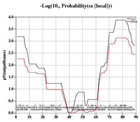 


- returns the rarray of expected probabilities of local insignificance of the pairwise sequence alignment ali_2seq. The Karlin and Altschul score probability values (option local ) or local ZEGA probabilities (see also Probability(i_, r_)) are calculated in multiple windows ranging in size from i_windowSize1 to w_windowSize2 (default values 5 and 20 residues, respectively). The exact formulae for the Karlin and Altschul probabilities (option local ) are given in the next section and the ZEGA probabilities are given in the Abagyan&Batalov paper. The window with the lowest probability value is chosen in each position. The array returned by this function can be used to color-code the regions of insignificant sequence-structure alignment in modeling by homology. One can use the Rarray(R_,ali_,seq_) function to project the array onto selected sequence.
To calculate an array of mean scores for each column of a multiple sequence alignments use the Rarray( ali [ exact ] ) function.
Example:

read alignment s_icmhome+ "sx"  # 2 seq. alignment 
 read pdb  s_icmhome+"x" 
 p= -Log(Probability(sx)) 
 display ribbon a_ 
 color ribbon a_/A -Rarray(p,sx,cd59)  
 # Rarray projects the alignment array to the sequence




 Probability ( seq_1  seq_2 [ i_windowSize1  i_windowSize2 ] )  

- returns a dot matrix of probabilities of local statistical comparison between the two sequences. This matrix contains local probability values that two continuous sequence fragments of length ranging from i_windowSize1 to w_windowSize2 have statistically insignificant alignment score , which means that the match is random. Visualization of this matrix allows one to see periodic patterns if sequence is compared with itself as well as identity alternative alignments. The formula is taken from the Karlin and Altschul statistics:
P= 1-exp(-exp(-Lambda*Sum(score in window)/K)), where Lambda and K are coefficients depending on the residue comparison matrix.
This example allows one to trace the correct alignment despite an about 100 residue insertion:

read pdb sequence "2mhb" 
 read pdb sequence "4mbn" 
 m=Probability(2mhb_a 4mbn_a 7 30) 
 print " pProbability: Min=" Min(Min(m)) "Max=" Max(Max(m)) 
 PLOT.rainbowStyle="white/rainbow/red" 
# show probability of the chance matching (comparable to the BLAST P-value) 
 plot area m display color={.2 0.001} transparent={0.2 1.} link grid 
# OR show -Log10(Probability)  
 plot area -Log(m,10) display color={0.7 3.} transparent={0. 0.7} link grid

---




Profile

function.


 Profile ( chem i_at1 i_at2 i_at3 i_at4 )  

 Profile ( chem selection )

 Profile ( v_tor {group|randomize} )

Returns torsion statistical profile predicted by graph Convolutional Neural Network (GCNN) trained on structures from Crystallography Open Database (COD) J Chem Inf Model. 2022 Dec 12;62(23):5896-5906. doi: 10.1021/acs.jcim.2c00790. Epub 2022 Dec 1.

 Profile ( alignment )  

- creates profile from an alignment

---




Property

 Property ( grob option )  

- returns various advanced grob properties as logical.

Available options:

• full -- dual in-out lighting of the grob
• surface -- whether only the front face of the triangles is shown (back faces culled)
• texture -- allow textures
• material -- allow materials
• grid -- (requires texture). Use only the fractional part of the texture coordinates (allows repetitive pattern textures)
• heavy -- grob lids on sliced surfaces

See also set property

Putarg

 Putarg( s_name s_value )

- adds a name-value pair to the list of ICM arguments. Returns no in case of error.

See Getarg .

---

Putenv

function to change or add value to environment.

 Putenv ( " s_environmentName = s_environmentValue " )

-returns a logical yes if the named shell-environment variable is created or modified.


 Putenv ( )  

- function to push the icm or icm-script arguments (see Getarg ) into the unix shell as shell arguments. Returns the number of set variables. To eliminate an agrument from the list, use the Getenv ( s_argName delete ) function.


Examples:

show Putenv("aaa=bbb") # change/add variable 'aaa' with value 'bbb' to environment 
show Getenv("aaa")     # check if it has been successful

See also: Existenv, Getenv, Getarg.

---




Radius

atomic radii (van der Waals, surface energy, and electrostatic).


 Radius (  as ) 

- returns the real array of van der Waals radii of atoms in the selection.
These radii are used in the construction of the molecular surface (skin) and can be found (and possibly redefined) in the icm.vwt file.

 Radius ( as  ball ) 

- returns the rarray of the graphical radii of the xstick or ball representation. Normally they are defined by the GRAPHICS.stickRadius parameter and GRAPHICS.ballStickRatio . They can be set to custom values with the set atom


 Radius ( as  surface ) 

- returns the rarray of the 'hydration' atomic radii.
These radii are used in construction of the solvent-accessible (surface) and can be found (and possibly redefined) in the icm.hdt file.


 Radius ( as  charge ) 

- returns the rarray of the 'electrostatic' atomic radii.
These radii are used for building the skin (analytical molecular surface) for electrostatic dielectric boundary calculation with electroMethod = "boundary element". These parameters can be found (and possibly redefined) in the icm.vwt file.

---




Random

[ Random string ]

evenly distributed random function.


 Random ( ) 

- returns a pseudo-random real in the range from 0. to 1.


 Random ( i_max ) 

- returns a pseudo-random integer distributed in [1, i_max ]


 Random ( i_min , i_max ) 

- returns a pseudo-random integer distributed in [ i_min , i_max ]


 Random ( r_min ,  r_max ) 

- returns a pseudo-random real evenly distributed in [ r_min , r_max ]


 Random ( r_min ,  r_max , i_n ) 

- returns a rarray [1: i_n ] with pseudo-random real values distributed in [ r_min , r_max ]


 Random ( r_mean ,  r_std , i_n , "gauss" ) 

- returns a rarray of i_n elements with normally distributed pseudo-random values. The mean and standard deviation are provided as the first two arguments


 Random ( r_min ,  r_max , i_nRows ,  i_nColumns ) 

- returns a matrix [1: i_nRows, 1: i_nColumns] with pseudo-random real values distributed in [ r_min , r_max]


 Random ( i_nRows,  i_nColumns,  r_min,  r_max ) 

- returns a matrix [1: i_nRows, 1: i_nColumns] with pseudo-random real values distributed in [ r_min, r_max ]

Examples:

print Random(5)            # one of the following: 1 2 3 4 or 5  
 print Random(2,5)          # one of the following: 2 3 4 or 5  
 print Random(2.,5.)        # random real in [2.,5.]  
 randVec=Random(-1.,1.,3)   # random 3-vector with components in [-1. 1.]  
 randVec=Random(3,-1.,1.)   # the same as the previous command  
 randMat=Random(-1.,1.,3,3) # random 3x3 matrix with components in [-1. 1.]  
 randMat=Random(3,3,-1.,1.) # the same as the previous command   
 Random(0., 1., 10, "gauss" ) # normal distribution

---




Random strings

 Random( I_lengths s_alphabet )

- returns an sarray of random strings of lengths specified in the I_lengths array. Strings are comprised from the characters specified in the s_alphabet. Alphabet specifications are the same as character set specifications in regular expressions: "A-Z", "\\w", "\\dA-Fa-f", "ACGT".

 Random( i_n S_words ) 

- returns an i_n element sarray consisting of the words specified in the S_words array repeated in random order.

Examples:

Random( Iarray(10,20) "\\dA-Z" ) # returns 10-element sarray with 20-character strings containing random digits and capital letters
Random( 100, {"rock","paper","scissors"} ) # returns 100-element sarray consisting of words "rock", "paper" and "scissors" in random order
Random( 100, Random( Iarray(10,3) "a-z" ) ) # returns 100-element sarray containing 10 random words from the "a-z" alphabet

Rarray

[ rarray sequence projection | Rarrayinverse | R property transfer via alignment | Rarray properties | RarrayAlignment ]

real-array function.


 Rarray ( i_NofElements ) 

- returns a rarray; creates zero-initialized rarray [1: i_NofElements]. You can also create an zero-size real array: Rarray(0) .


 Rarray ( i_NofElements,  r_Value ) 

- returns a rarray [1: i_NofElements ] with all elements set to r_Value.


 Rarray ( i_NofElements,  r_From,  r_To ) 

- returns a rarray [1: i_NofElements ] with elements ranging from r_From to r_To.


 Rarray ( r_From,  r_To , r_step ) 

- returns rarray of equally spaced numbers from r_From to r_To. Example:

Rarray( 3.1, 15. 0.1)




 Rarray ( iarray ) 

- converts iarray into a rarray.


 Rarray ( sarray ) 

- converts sarray into a rarray.

 Rarray ( sarray s_patternForValue1 ) 

- converts sarray into a rarray of 1. and 0. The value is 1. if an element if an array matches the string. E.g. Rarray({"M","W","M","E","W"},"M") # returns {1. 0. 1. 0. 0.}

 Rarray ( R n_significantDigits ) → R_rounded

- rounds the input array to the specified number of significant digits. If n is out of bounds ( less than zero or more than 12, the function switches to the default of 2.


 Rarray ( M [ i_flag ] ) 

- extracts different groups of elements of the matrix and casts them into a rarray. There are seven (7) possibilities for a matrix n rows by m columns:
1. all elements by rows (the default) , n*m
2. all elements by columns, n*m
3. the upper triangle with diagonal, n(n+1)/2
4. the lower triangle with diagonal, n(n+1)/2
5. the diagonal elements, n
6. the upper triangle without diagonal elements, n(n-1)/2
7. the lower triangle without diagonal elements, n(n-1)/2

Examples:

a=Rarray(54)                     # create 54-th dimensional vector of zeros 
 a=Rarray(3,-1.)                  # create vector {-1.,-1.,-1.} 
 a=Rarray(5,1.,3.)                # create vector {1., 1.5, 2., 2.5, 3.} 
 a=Rarray({1 2 3})                # create vector {1. 2. 3.} 
 a=Rarray({"1.5" "2" "-3.91"})    # create vector {1.5, 2., -3.91} 
# 
 M=Matrix(2);M[2,2]=2;M[1,2]=3 
 Rarray( M ) 
 Rarray( M 1 ) 
 Rarray( M 2 ) 
 Rarray( M 3 ) 
 Rarray( M 4 ) 
 Rarray( M 5 ) 
 Rarray( M 6 ) 
 Rarray( M 7 )




rarray sequence projection

 Rarray ( R_ali  ali_from { seq | i_seqNumber } ) 


- returns a projected rarray. The R_ali rarray contains values defined for each position of alignment ali_from. The function squeezes out the values which correspond to insertions into sequence seq_, that is, in effect, projects the alignment array R_ali onto sequence seq_. E.g. for the residue conservation: Rarray( Rarray( alig ), alig , myseq ) -

Projecting from one sequence to another sequence via alignment.
Let us imagine that we have two sequences, seq1 and seq2 which take part in multiple sequence alignment ali . The transfer of property R1 from seq1 to seq2 can be achieved via two transfers :
1. seq1 to ali : RA = Rarray( R1 seq1 ali r_gapValues )
2. ali to seq2 : R2 = Rarray( RA ali seq2 )
Now R2 has the same dimension as seq2. Values aligned with seq1 are transferred by alignment, other values are set to r_gapValues .
See also:

String( s_,R_,ali_,seq_ )	function to project strings
Rarray( R_seq seq_ ali_to r_gapDefault )	function to project from sequence to alignment
Probability()	function




Reversing the order of elements in an array

 Rarray ( rarray reverse ) 


- converts input real array into an rarray with the reversed order of elements. Example:

Rarray({1. 2. 3.} reverse)  # returns {3. 2. 1.}




Transfer real sequence properties by alignment

 Rarray ( R_seq { seq | i_seqNumber } ali_to  r_gapDefault ) 


- projects the input rarray from seq_ to ali_to (the previous function does it in the opposite direction). The R_seq rarray contains values defined for each position of the sequence seq_. The function fills the gap positions in the output array with the r_gapDefault values.
Combination of this and the previous functions allow you to project any numerical property of one sequence to another by projecting the r1 property of seq1 first to the alignment and than back to seq2 (e.g. Rarray( Rarray(r1,seq1,a,99.) , a, seq2) ).
This function can also be used to determine alignment index corresponding to a sequence index. Example:

read alignment s_icmhome+"sh3" 
t = Table(sh3) 
group table t Count(Nof(t)) "n" append  # add a column with 1,2,3,.. 
show t  # t looks like this: 
 #>T t 
 #>-cons--------Fyn---------Spec--------Eps8-------n--- 
    " "         0           1           1          1 
    " "         0           2           2          2 
    " "         0           3           3          3 
    " "         0           4           4          4 
    .           1           5           5          5 
 ... 
t2forFyn =  t.Fyn == 2   # table row for position 2 in seq. Fyn 
t2forFyn.n               # corresponding alignment position


See also the String( s_,R_,seq_,ali_,s_defChar ) function to project strings.



Assign arbitrary amino-acid property to a sequence

 Rarray ( sequence  R_26resProperty ) 


- returns a rarray of residue properties as defined by R_26resProperty for 26 residue types (all characters of the alphabet) and assigned according to the amino-acid sequence.
Example with a hydrophobicity property vector:

s= Sequence("TTCCPSIVARSNFNVCRLPGTPEAICATYTGCIIIPGATCPGDYAN") # crambin sequence 
# 26-dim. hydrophobicity vector for A,B,C,D,E,F,.. 
 h={1.8,0.,2.5,-3.5,-3.5,2.8,-.4,-3.2,4.5,0.,-3.9,3.8,1.9,-3.5,.0,-1.6,-3.5,-4.5,-.8,-.7,0.,4.2,-.9,0.,-1.3,0.} 
 hs=Rarray(s,h)              # h-array for each sequence position 
 hh = Smooth(Rarray(s,h), 5) # window average




Calculating array of alignment strength values for each column

 Rarray ( ali  [ simple|exact ] ) 


- returns a rarray of conservation values estimated as mean pairwise scores for each position of a pairwise or multiple alignment. The number is calculated as the sum of RESIDUE_COMPARISON_VALUES over n*(n-1)/2 pairs in each column. The gapped parts of an alignment are considered equivalent to the 'X' residues and the comparison values are taken from appropriate columns.
Option exact uses raw residue substitution values as defined in the comparison matrix These values can be larger than one for the residues the conservation of which is important (e.g. W to W match can be around 3. while A to A match is only about 0.5.
By default (no keyword) the matrix is normalized so that two identical residues contribute the replacement value of 1. and two different but property-similar amino acid contributed values from 0. to 1. depending on the residue similarity.
If option simple is specified, each pair with identical residues contributes 1. while each pair of different amino-acids contributes 0. The resulting total of pairwise similarities d calculated for n(n-1)/2 pairs is then converted into the conservation value with the following equation: c = ½(1+ √(8·d +1) ) (a solution of the equation n² - n = 2d ) and further divided by the number of sequences in the alignment

The values returned with both simple option and the default are therefore between 1/n (all residues are different) and 1.
To project the resulting array to a specific sequence, use the Rarray( R_ ali_ seq_ ) function (see above).
To calculate conservation with respect to a particular set of residues in a structure, use the Score( rs_ [ simple ] ) function.

To project the conservation onto a 3d chain with its linked sequence in alignment use the Rarray( R_conserv alignment seq3d) projection function. e.g.
Example:

read alignment s_icmhome+"sh3" 
show Rarray(sh3) 
# 
a=Rarray(sh3 simple)  # a number for each alignment position 
# to project a to a particular sequence, do the following 
b=Rarray(a,sh3,Spec)  # a number for each Spec residue 
String(Rarray(a, sh3, Spec ))//String(Spec)   # example

See also:

•  Score( ali [simple])

•  Entropy( ali [simple|info])

---




Real function

generally converts things to a real.


 Real ( integer ) 

- converts integer to real number.


 Real ( string ) 

- converts string to real number. The conversion routine ignores trailing non-numerical characters.
Examples:

s = "5.3"         
 a = Real(s)      # a = 5.3  
 s = "5.3abc"     # will ignore 'abc'    
 a = Real(s)      # the same, a = 5.3

See also: Toreal

---

Remainder function.

Returns the remainder; similar to, but different from the Mod function.

function	description	example
Remainder(x,y)	brings x to [-y/2 , y/2] range	Remainder(17.,10.) → -3.
Mod(x,y)	brings x to [0 , y] range	Mod(17.,10.) → 7.




 Remainder ( i_divisor, [ i_divider ] ) 

- returns the integer


 Remainder ( r_divisor, [  r_divider ] ) 

- returns the real remainder r = x - n*y where n is the integer nearest the exact value of x/y; if | n-x/y|=0.5 then n is even. r belongs to [ -|y|/2, |y|/2 ] range


 Remainder ( iarray, [  i_divider ] ) 

- returns the iarray of remainders (see the previous definition).


 Remainder ( rarray, [  r_divider ] ) 

- returns the rarray of remainders.
The default divider is 360. (real) or 360 (integer) since we mostly deal with angles.
Examples:

read object s_icmhome+"crn.ob"
              # transform angle to the standard  
              # [-180., 180.] range. (Period=360 is implied)  
 phi=Remainder(Value(v_//phi))
 
              # we assume that you have two objects 
              # with different conf. of the same molecule

---

Reference

 Reference( seq [ s_fieldName ] ) 

- returns the swissprot database reference if available. It is possible to specify the requested field name; the default is "DR".

---

Replace

[ Replace exact | Replace simple | Replace regexp | Chemical replace ]

- text substitution function.

 Replace( s|S s_regexp s_by regexp [i_field=0] ) → s|S  

(regular expressions, and case-sensitivity, - see below).


 Replace ( s_source  s_icmWildcard  s_replacement ) 

- returns a string, which is a copy of the source string with globally substituted substrings matching s_icmWildcard by the replacement string s_replacement.
Example:

a=Replace(" 1crn "," ","")  # remove empty space




 Replace ( s_source  S_fromArray  S_toArray ) 

- make several replacements in a row. The size of the two arrays must be the same.
Example which generates a complimentary DNA strand (actually there is a special function Sequence( seq_, reverse ) which does it properly).

invertedSeq = String(0,1,"GTAAAGGGGTTTTCC")  # result: CCTTT.. 
 complSeq=Replace(invertedSeq,{"A","C","G","T"},{"T","G","C","A"}) 
# result: GGAAA...




 Replace ( s_source  S_fromArray  s_replacement ) 

- replace several strings by a single other string. If s_replacement is empty, the found substrings will be deleted.
Example which generates a complimentary DNA strand:

cleanStr=Replace("XXTEXTYYTEXT",{"XX","YY"},"")




 Replace ( S  s_icmWildcard  s_replacement ) 

- returns a sarray with globally substituted elements (the original sarray remains intact).
Examples:

aa={"Terra" "Tera" "Teera" "Ttera"} 
 show column aa Replace(aa "er?" "ERR") Replace(aa "*[tT]" "Shm")




 Replace (  S  S_fromArray  S_toArray )  or

 Replace (  S  k_translation_name-val_collection [s_nonMatchFormat])) 

- returns a sarray with multiple substitutions.


 Replace (  S  s_icmWildcard  s_replacement ) 

- returns a sarray with multiple substitutions to a single string.

Replace a matching element of an array with another string.

 Replace( S s_completeString s_by exact ) → S

Search a string array and find an element which matches the full s_completeString, e.g. the "never again" element of S will only be matched with the "never againg" string, but not with "never" .

A straight forward substitution. Replace without any interpretation of the search string.

 Replace( s|S s_whatAsIs s_byAsIs simple ) → s_|S

In this case there is not intepretation of the query string. The first occurrence of it is replaced with the second argument. Example:

s="a[b]()c"
Replace(s,"[b]","()$",simple) # no intepretation

Replace using regular expressions

 Replace( s|S s_regexp s_by regexp [i_field = 0] ) → s|S

- replace the s_regexp in the source string or array by s_byRegexp using regular expressions. The latter is a string which may contain back-references.

Example: case-insensitve replacements:

Replace("bla 1"//"Bla 2"//"BLA 3" , "(?i)bla ","") # get rid of bla

Example:

read string "t.html"
  s_out = Replace( s_out, "(?n)<i>(.*?)</i>", "<b>\\1</b>" regexp )   # replace italic with bold
  s_out = Replace( s_out, " +", " ",regexp )   # replace multiple spaces with a single on

Note that "(?n)" modifier is needed to make '.' match newline too.

Dehtml-tagging of the html text in a string or a string array:Prep work in html conversion is usually this: <> S = Replace( S, "
","\n", exact) S = Replace( S, "

","\n\n", exact) S = Replace( S, " "," ", exact) # finally remove all tags S = Replace( S, "<.*?>","",regexp) <>

Example in which we remove href html tags from a column in a table :

read table html "http://pfam.sanger.ac.uk/search/keyword?query=sh2" name = "sh2t"
sh2t.ID = Replace(sh2t.ID, "<.*?>","",regexp)

Chemical replace

 Replace( chem , s_smartFROM, s_smileTO [exact] )

Finds a chemical pattern containing one of several Rn groups and replaces the pattern to the s_smileTO pattern according to the matching R-groups. Note that all atoms except the ones connected to the R-groups in s_smartFROM pattern will only match exactly the same local pattern.

The molecules will be redrawn in 2D after the replacement. The exact option will supress the redrawing if the number of atoms in the FROM and TO patterns is the same.

Example in which we created a newe table tt with a modified column:

read table mol "drugs.sdf"
add column tt Replace(drugs.mol, "[R1]C(=O)O","[R1]C(=O)OC")

See also:

 modify chemarray s_pattern s_repl [exact]

will modify in place. This replacement can be done only for the "terminal" fragments (one attachment point)

 `Trim-chemical{Trim} ( X [s_smart] ...) 

will iteratively delete selected atom pattern, e.g. "[*;D1]"

---

Res

residue selection function.


 Res ( {  os |  ms | rs | as } [ append ] ) 

 Res ( {  rs [ append ] ) 


- selects residue(s) related to the specified objects ( os_), molecules ( ms_) or atoms ( as_), respectively. Option append extends the selection with the terminal residues (like Nter and Cter in peptides)
Examples:

show Res( Sphere(a_1/1/* 4.) )   # show residues within 4 A  
                                  # vicinity from the firsts one


See also: Atom ( ), Mol ( ), Obj ( ).


Res(ali ..): from sequence positions in sub-alignment to residue selection

 Res (  ali  { seq | i_sequence } ) 

- returns residue selection corresponding to the aligned positions of the specified sequence. The sequence can be specified by its order number in the alignment (e.g. 1crn_m in the example below has number 1 ), or by name.

---




Resolution

- returns the X-ray resolution in Angstroms.


 Resolution ( ) 

- returns the real resolution of the current object.


 Resolution ( os_object ) 

- returns the rarray X-ray resolutions for the specified objects. The resolution is taken from the PDB files.
Examples:

sort object Resolution(a_*.) # resort objects by resolution
 res=Resolution(a_1crn.)[1]
 print "PDB structure 1crn: resolution = ", res, " A"




 Resolution ( s_pdbFileName  pdb ) 

- returns the real resolution of the specified pdb-file. The function returns 9.90 if resolution is not found.


 Resolution ( T_factors [  R_6cell ] ) 

- returns the rarray of X-ray resolution for each reflection of the specified structure factor table. The resolution is calculated from h, k, l and cell parameters taken from R_6cell or the standard defCell shell rarray.
Example:

read factor "igd"   # read h,k,l,fo table from a file 
 read pdb "1igd"     # cell is defined there 
 defCell = Cell(a_)  # extract the cell parameters from the object 
 group table append igd Resolution(igd) "res" 
 show igd

See also: set resolution

---




Ring

 Ring( as )

- returns logical yes all atoms from the selection belong to one ring

 Ring( vs )

- returns subset of input variable selection which belongs to one ring

 Ring( chemical )

- returns chemical array of ring system(s)

 Ring( chemical simple )  

- returns chemical array of the smallest set of smallest rings (SSSR) Example:

show Smiles( Ring( Chemical("C(=CC=CC1C(=CC=C(C2C3)C=CC=3)C=2)C=1" ) ) unique )
show Smiles( Ring( Chemical("C(=CC=CC1C(=CC=C(C2C3)C=CC=3)C=2)C=1" ) simple ) unique )

---

Rfactor

crystallographic R-factor.


 Rfactor ( T_factors ) 

- returns the real R-factor residual calculated from the factor-table elements T_factors.fo and T_factors.fc. Reflections marked with T_factors.free = 1 are ignored.

---




Rfree

crystallographic free R-factor.


 Rfree ( T_factors ) 

- returns the real R-factor residual calculated from the factor-table elements T_factors.fo and T_factors.fc. Only reflections marked with T_factors.free = 1 will be used.

---




Rmsd

Root-Mean-Square-Deviation function.


 Rmsd ( { iarray | rarray | matrix | map } ) 


- returns the real standard deviation estimate (sigma) from the estimated mean for specified sets of numbers. This function returns the unbiased estimation of standard deviation with Bessel's correction according to this formula: s = √(∑(xᵢ-μ)²/(n-1) ), where μ is the sample mean.

 Rmsd ( Rn Wn ) 

- returns the real weighted rmsd and weighted mean as r_out according to this formula:

xw = Sum(w[i]*x[i])/Sum(w[i])  # the weighted mean
np    # is the number of non-zero weights
sdw2 = Sum(w[i]*(x[i]-xw)^2) / (((np-1)/np)*Sum(w[i]))
sdw  = Sqrt(sdw2)





 Rmsd ( as_tetheredAtoms ) 

returns the real root-mean-square-deviation of selected atoms from the atoms to which they are tethered . The distances are calculated after optimal superposition according to the equivalences derived from tethers (compare with the Srmsd( as_ ) function which does not perform superposition ). This function also returns the transformation in the R_out array.


 Rmsd ( ms_select1 ms_select2 chemical [output] ) 

- returns the real root-mean-square distance between two selected chemical (hetero) molecules after an optimal chemical superposition via graph-matching is performed. In this mode atom equivalence can be found either by substructure search or (if none of molecules is substructure of other) by common substructure search algorithm. Other feature of chemical mode is that it enumerates topologically equivalent atoms to find best superposition. The maximal common substructure will be used for the calculation. Option output will produce R_2out array with individual deviation for the matched pairs. Rmsd(R_2out) will essentially be the overall Rmsd, but one will be able to measure the maximal and median deviation as well.

See also Srmsd( ms1 ms2 chemical ) and superimpose command.

 Rmsd ( chemarray ms_select2 [pharmacophore] ) 

- returns real array of root-mean-square distances between each element of chemarrayand ms_select2.

pharmacophore toggles pharmacophore superposition. ms_select2 - pharmacophore template.

 Rmsd ( as_pharmTemplate as_select2 pharmacophore ) 

- returns the real root-mean-square distance between pharmacophore points of as_pharmTemplate and as_select2after an optimal superposition of as_pharmTemplate

See also: find pharmacophore , show pharmacophore type , makePharma

 Rmsd ( as_select1 as_select2 [ { { ali|align } | exact } ] ) 


- returns the real root-mean-square-distance between two aligned sets after these two sets are optimally superimposed using McLachlan's algorithm.
Virtual atoms. Be default, the first two virtual atoms ( vt1 and vt2 ) are automatically excluded from both selections unless the virtual option is explicitly specified.
The optional third argument defines how atom-atom alignment is established between two selections (which can actually be of any level atom selection `as_ , residue selection `rs_ , molecular selection `ms_ , or object selection `os_ , see alignment options). Number of equivalent atom pairs is saved in i_out . Two output selections as_out and as2_out contain corresponding sets of equivalent atoms. This function also returns the transformation in the R_out array.
See also: superimpose and Srmsd ().
Examples:

read pdb "1mbn"                          # load myoglobin  
 read pdb "1pbx"                          # load alpha and beta 
                                          # subunits of hemoglobin  
 print Rmsd(a_1.1 a_2.1 align)            # myo- versus alpha subunit 
                                          # of hemo- all atoms 
 print Rmsd(a_1.1//ca a_2.1//ca align)    # myo- versus alpha subunit 
                                          # of hemo- Ca-atoms 
 
 print Rmsd(a_1./4,29/ca a_2.1/2,102/cb exact) # exact match

---




Rot

rotation matrix function.


 Rot ( R_12transformVector ) 

- extracts the 3x3 rotation matrix from the transformation vector.


 Rot ( R_axis ,  r_Angle ) 

- returns matrix of rotation around 3-dimensional real vector R_axis by angle r_Angle. To solve the inverse problem, i.e. calculate the angle from a transformation, use the Axis( R_12 ) function which returns the angle as r_out .
Examples:

#  rotate molecule by 30 deg. around z-axis  
 rotate a_* Rot({0. 0. 1.},30.)




 Rot (  R_3pivotPoint  R_3axis ,  r_Angle )  


- returns rarray of transformation vector of rotation around 3-dimensional real vector R_axis by angle r_Angle so that the pivotal point with coordinates R_3pivotPoint remains static.
Examples:

# rotate by 30 deg. around {0.,1.,0.} axis through the center of mass 
 nice "1crn" 
 R_pivot = Mean(Xyz(a_//*)) 
 transform a_* Rot(R_pivot,{0. 1. 0.}, 30.)

---




Sarray

[ Sarray index ]

sarray function.


 Sarray ( integer ) 

- returns empty sarray of specified dimension


 Sarray (  integer  s_Value ) 

- returns sarray of specified dimension initialized with s_Value

 Sarray (  integer  S_ids ) 

- returns sarray of unique strings using the ID seeds. Examples:

Sarray(10,Sarray(0)) # ID1 ID2 etc.
Sarray(10,{"A"})
Sarray(10,{"A","B","C"})
#
read csv header name='b' s_icmhome + "bnames.csv" # 2K baby names
Sarray(10000,Shuffle(Unique(b.name,sort)))  # useful for generating identifiers in tables

 Sarray (  s_wildCard  directory [simple|all] ) 

- returns sarray of file names with full path to them. With 'simple' option only file names are stored in the result array. all toggles recursive search in sub-folders.

Example:

Sarray( "*.pdb" directory )
  Sarray( "/home/user/*.ent*" directory )
  if (Nof( Sarray("*.png") )==0) print "No images found"

 Sarray ( string ) 

- converts the input string into a ONE-dimensional sarray . To split a string into individual lines, or to split a string into a sarray of characters, use the Split() function.


 Sarray ( iarray|rarray|sarray ) 

- converts input arrays into an sarray.

 Sarray ( sarray [32] hash ) 

- generates 32 char or 26 char MD5 based has string. Example in which we create a unique chemical id:

add column t Chemical({"C1CCCC1","CCO"})
  add column t Sarray(Smiles( t.mol unique cistrans ), 32 hash)





 Sarray ( rs [ { append | name | residue } ]) 

- converts input residue selection into an sarray of residue ranges, e.g.: {"a_a.b/2:5", "a_a.b/10:15",..} or with option residue into an array of individual selections (see also Name( rs full ) . Options:
• append : will merge residue ranges
• name : will return a string array of residueName residueNumber records
• residue : will return an array of selection strings a_obj.mol/residueNumber records

Example:

Sarray(a_/2,4:5 name) 
 #>S string_array 
 def.a1/ala2 
 def.a1/trp4 
 def.a1/glu5 
Sarray(a_/2,4:5 residue) 
 #>S string_array 
 def.a1/2 
 def.a1/4 
 def.a1/5 
Field(Sarray(a_/2,4:5 name),2,"/") # extract residues 
#>S string_array 
 ala2 
 trp4 
 glu5


The l_showResCodeInSelection system logical controls if one-letter residue code is printed in front of the residue number ( e.g. a_/^F23 instead of a_/23 ).
See also:
• Name( rs full ) : preferred way to generate arrays of residue selection strings
• String( rs_ ) which returns one string;
• Label( rs_ | as_ ) which will format the output string according to the resLabelStyle or atomLabelStyle preference.
• l_showResCodeInSelection



 Sarray ( stack, vs_var )  

- creates a string representation of all the conformations in the stack Variable selection allows one to choose the conformational feature you want. Character code:
Backbone (phi,psi pairs):
• 'B': -200 < phi < -80 , 140 < psi < 200
• 'A': -101 < phi < -24 , -81 < psi < 4
• 'g': -169 < phi < -15 , -64 < psi < 54
• 'd': -211 < phi < -5 , 8 < psi < 136
• 'L': 24 < phi < 101 , -4 < psi < 81
• '_': the rest

Sidechain (chi1):
• 'M': -120 <= xi1 < 0
• 'P': 0 <= xi1 < 120
• 'T': 120 <= xi1 < 240

Example:

show Sarray(stack,v_/2:10/x*)      # coding of side-chain conformations 
 show Sarray(stack,v_//phi,psi)     # backbone conformation character coding 
 show Sarray(stack,v_/2:10/phi,PSI) # character coding of a chain fragment

(Note use of special PSI torsion in the last example.)
Other examples:

ss=Sarray(5)       # create empty sarray of 5 elements  
 ss[2]="thoughts"   # assign string to the second element of the sarray  
 
 sa=Sarray("the first element") 
 
 show Sarray(Count(1 100)) # string array of numbers from 1 to 100




 Sarray (sarray reverse ) 

- Reversing the order of elements in an sarray
- converts input sarray into an sarray with the reversed order of elements. Example:

Sarray({"one","two"} reverse)  # returns {"two","one"}


See also: Iarray( I_ reverse ), Rarray( S_ reverse ), String(0,1,s)


 Sarray ( sarray i_from i_to ) 


returns sarray of substrings from position i_from to position i_to . If i_from is greater than i_to the direction of substrings is reversed. Example:

a={"123","12345"} 
Sarray(a,2,3) 
 {"23","23"} 
Sarray(a,5,2) 
 {"32","5432"}




Getting selected entries from index table

this function allows one to get


 Sarray ( T_index ) 

- returns sarray of index table elements
Example:

read index "myindex"
S = myindex[2:8]
S[1]

See also: write index

---




Score

[ Score overlap | Score chemset | Score torsion | Score apf | Score model | Score predictions | Score sequence | Score conservation | Score alignment ]

function. Summary:

Score( <R_X> <R_Y> ) => r [-1.:1.] # overlap between two distributions
 Score( <R_Ei> <R_Di> <wE> <wD> ) => <r> # prediction quality
 Score( <I_keys1> <I_keys2> <nBits>|<R_bitWeights> [simple] ) => M # Tanimoto distances
 Score( <seq1> <seq2> [new|nucleotide|simple] ) => <R_scores>
 Score( <seqArray[n]> ) => Mnn_alignedScore
 Score( <i_len> <r_probability> [comp_matrix|similarity|identity] ) => <r_>
 Score( <ali2> [area|sort|comp_matrix|similarity|identity  [<i_alnLength>] ] ) => r # see also Distance (<ali>), and Rarray(<ali>) 
 Score( <X_n> <X_m> [[<R_Wn> <R_Wm>] <r_minScore> (0.4) [<r_steepness>(6.)]] set ) => r_inter_set_score [0:1]
 Score( <X_3D_n> [<X_3D_m>] field|similarity|distance ) => <M_nxm APF_scores> # needs Chemical(<as> exact hydrogen)
 Score( <X_3D_n> torsion ) => <R_Free_Strain> # 
 Score( <rs_n> [simple|info|comp_matrix] ) => <R_n_conserv_scores> # info is entropy
 Score( <rs_n> <seq_n> ) => <r_score_without_alignment>
 Score( <rs_n> <seq_n> all ) => <T_sel_scores_seqids>
 Score( <model> full|test [<s_stats>] ) => <r_learnStatistics>
 Score( predict <R|I_obs> <R|I_pred> [<R_weights>] ) => <R_allRegression_or_Classification_Stats>




A measure of overlap between two arrays

 Score ( R_1,  R_2 ) → r_overlapMeasure

- returns the real measure of overlap between two real arrays. This measure varies between -1 and 1.. (all values of R_1 are smaller than all values of R_2) and +1. (all values of R_1 are greater than all values of R_2) and may serve as a ranking criterion.
Examples:

show Score({1. 2. 5. 3.} {3. 1.5 1.5 5.})  # 0. perfectly overlapping arrays 
 show Score({2. 5. 3.} {1. 1.5 0.5})        # 1. no overlap R_1 > R_2 
 show Score({1. 1.5 0.5} {2. 5. 3.})        # -1. no overlap R_2 > R_1 
 show 1.-Abs(Score({1. 3. 2.5} {2. 5. 3.})) # relative overlap between R1 and R2

Similarity score between two sets of ligands

 Score( X_n X_m [[R_Wn R_Wm] r_minScore (0.3) [r_steepness(6.)]] set ) → r_sim_score [0:1]

This function returns a similarity (0. to 1.) between two sets (arrays) of chemicals. It is calculated as N_AB /( N_AA + N_BB - N_AB ), where N is an effective number is similar compounds calculated as weighted sum of sigmoidly transformed similarities to the power of one half. The original similarity measure is transformed by a sigmoid starting from r_minScore (0.) and ending at 1. The mid point of the sigmoid is at 0.5*(1+ r_minScore ) . A general form of the sigmoid before it is shifted and squeezed is 1./(1.+exp(-b*t)) where b is r_steepness . Arguments:

• X_n , X_m : two chemical arrays of size n and m
• W_n , W_m : weights assigned to the chemicals
• r_minScore> (0.3) , first non-zero value of the shifted sigmoid.
• r_steepness (6.) ; steepness of 0. corresponds to the linear function between 0. and 1.
Other returned values:
• r_out : N₁₁
• r_2out : N₂₂
• r_3out : N₁₂
Example:

Score( t.mol tt.mol set )

Free Strain for 3D molecules

 Score( X_3Dn torsion ) → R_n_free_strain 

returns free strain(s) for a set of 3D molecules

Calculated as:

= -Sum(Log(Probability_Tors[i])

where

Probability_Tors[i] = Sum( prof[k]*Exp(-d*d) ) k : 1:36 # 36 bins d : current_torsion_bin-k # distance in bins between current torsion angle bin and k

The result includes entropy component : if there are three equal depth minima, even at the bottom of any of them there will be an offset penalty corresponding to entropy loss associated with locking out two of the three minima.

APF similarity between superimposed ligands in 3D

 Score( X_3Dn [X_3Dm] field|similarity|distance ) → M_nxm apf_scores 

returns all pairwise APF scores between 3D chemical arrays. Two prerequisities:

• a superimposed set of ligands in a chemical 3D array
• and APF parameters loaded with the

  read pmf s_icmhome + "APF"

An array can be generated with Chemical ( ms exact ) function. If one array is provided an n by n matrix with all pairwise scores is calculated. The options:
• field : returns raw (negative for similar atom pairs) pairwise APF similarity scores Sij
• similarity : returns normalized APF similarity calculated as S_ij_sim = |Sij|/Sqrt(|Sii*Sij|). (we change the signs on Sij values to make it positive if necessary). The similarities are 1. for self-comparison and numbers less for different molecules.
• distance : returns chemical distance calculated as 1. - normalized_similarity .

Example:

build string "H"
build string "W"
build string "A"
add column t Chemical(a_*. exact hydrogen ) name="mol"
read pmf s_icmhome+"APF"
show Score(a_1. a_2. field)
sf = Score( t.mol field )
ss = Score( t.mol similarity )
sd = Score( t.mol distance )
CS = Rarray( ss 6 )  # off diagonal elements 
Mean(CS)             # average similarity

If the two sites (or atoms sets) are not superimposed, use the siteSuperAPFas1 as2 exact macro which makes the superposition and returns the un-normalized score. The normalized score can be returned after converting the superimposed selections into a 3D chemical array with the Chemical( as exact ) function Alternatively, the normalization can be done directly by the above formula ( S_ij = |Sij|/Sqrt(|Sii*Sij|) if self-scores are calculated.

Quality measures of a regression or classification model.

 Score ( model [ test | full ] s_stats ) → r_PredictionQuality 

Categorical or class prediction (e.g. Bayesian classifier). If each data record has a label which can be either positive or negative (say, 1, or -1) then the success of a prediction method can be measured by the following measures:

measure	abbreviation/formula	description
"tpos"	TP	number of true positives
"fneg"	FN	number of false negatives
"fpos"	FP	number of false positivers
"tneg"	TN	number of true negatives
"accuracy"	Q=(TP+TN)/(TP+TN+FP+FN)	fraction of correctly predicted label assignments
"sensitivity"	TP/(TP+FN)	fraction of correction predicted positive labels
"specificity"	TN/(TN+FP)	fraction of correction predicted negative labels
"mathews"	(TP*TN-FN*FP)/Sqrt((TP+FN)(TP+FP)(TN+FN)(TN+FP))	Mathews correlation
"precision"	PR=TP/(TP+FP)
"recall"	RE=TP/(TN+FP)	same as sensitivity
"f1"	2*PR*RE/(PR+RE)

Note that only "acuracy", and "mathews" are overall measures symmetrical with respect to the label. Frequently a method is characterized by an area under a recall - precision curve.

Quality measures to evaluate a regression method predicting numerical values, e.g. Partial Least Squares, or Kernel Regression.

measure	formula	description
"r2"	r=Mean((X-))/(Stdev(X)*Stdev(Y)) ; r2=r*r	correlation squared
"rmse"	Sqrt(Sum((Xpred-Xobs)^2 )/N)	root-mean-squared error
"expavg"




Scoring prediction quality from an array of errors and predicted scores

 Score ( R_En,  R_Dn, wE, wD ) → r_PredictionQuality 


Evaluates the quality of submitted multiple predictions for a unknown outcome. The submitted provies R_En , the evaluator evaluates R_Dn from the correct answer, then plugs in the weights and calculates the quality. The Q (quality)-value of predicted "energies" R_En for n - states, by comparing predicted energies with the deviations R_Dn from the correct answer. In essence we are doing the following:
• starting from distances (e.g. RMSD) from the correct answer Di (Di >=0.)
• calculating their well-behaved and inverted version, exp( -w*D ) [0., 1.]
• calculating the normalized Boltzmann average if the previous similarity measure
• taking -Log of the previous average
For example, if you predicted n conformations with energies E[n] and calculated RMSD deviations D[n] for each of those conformations from the correct conformation, the quality of your prediction will be calculated by this function.
The Q-value is calculated as follows:
Q = - Log( Sum( exp(- wE#(Ei-Emin) -wD*Di )) / Sum(exp(- wE#(Ei-Emin))) )
The best Q -value is 0. (it means that zero deviation (Di=0.) correspond to the best energy and the energy gap is large. The weighting factors wE and wD can be used to change the relative contributions of energies and deviations.


Aligning and scoring pairwise sequence alignment

 Score ( sequence1,  sequence2 ) 


- returns the real score of the Needleman and Wunsch alignment.
Each pair of aligned residues contributes according to the current residue comparison table, which is normalized so that the average diagonal element is 1. Insertions and deletions reduce the score according to the gapOpen and gapExtension parameters. Approximately, the score is equal to the number of residue identities.
To calculate an array of mean scores for each column of a multiple sequence alignments use the Rarray( ali [ exact ] ) function. i_out returns the number of identical residues.
Examples:

read sequence msf s_icmhome+"azurins.msf"
 a = Score( Azur_Alcde Azur_Alcfa ) # it is around 90.

 Score ( seq_n_long,  seq_m_short simple )  → R_n-m+1_scores

returns an array of scores of sliding no-gap sequences.

 Score ( seq_n,  rs_N )  → r_no_gap_score

 Score ( seq_n,  rs_N all )  → T_N-n_scores_ids_for_all_frames

these two functions return the match or no-gap-alignment score for one frame or multiple frames with the all option.

The second function template returns a table with the following columns: i (relative number), nu (first residue number), sl (fragment selection string), se (the first residue code), sc (normalized alignment score divided by the sequence selfscore and multiplied by 100., id (sequence identity), sf (relative surface area), ss ( relative non-loopsecondary structure ). id , sf , ss range from 0. to 100. % . Make sure to assign the secondary structure and calculate the atomic surface areas before you fun the Score(.. all ) function. Example:

build string "ASDFY"
a=Sequence("SDF")
assign sstructure a_/A
show surface area 
t = Score( a_/A a all)
show t

See also: Distance( ).


Conservation score per residue from an alignment projected to a structure.

 Score ( rs, [ simple | comp_matrix | info ] )  

Setup: a multiple sequence alignment, one of the sequences is linked to a structure, you may want to color residues by conservation or other measure of a column in an alignment. For a straight conservation value for each position in an alignment see Rarray( ali ) The function returns the rarray of alignment-derived conservation values for the selected residues. For each residue Ri in the residue selection rs_ the following steps are taken:

• a column is extracted from a linked N-sequence alignment ( see the link command )
• Si = Sum( Cij )/N where j=1,..N and Cij is the residue comparison value
• simple mode: Cij = 1. for two identical residues and 0. otherwise . It is also the default.
• comp_matrix (also the default) mode: Cij is taken from a normalized comp_matrix . Its elements are calculated as Cij_norm = Cij/Sqrt(Cii*Cjj) with the negative elements set to zero. The sum, d, of normalized positive similarity values c_ij is then converted to the conservation value of (1/2·n_seq) √(8d+1) .
• info (inverse information entropy mode): Cij = 1./(1.+Entropy), where Entropy= -Sum((fj)Log(fj)). The elements after normalization range from 0. (no conservation, 1. conservation).
The default mode shows positions with residues of the same type as more conserved than positions with residues of different types.
Example in which we compare conservation on the surface and in the core:

read alignment s_icmhome+"sh3.ali" 
  read pdb "1fyn" 
  make sequence a_a 
  group sequence sh3 
  align sh3 
  display ribbon 
  color ribbon a_a/A Score( a_a/A simple ) 
  show surface area 
  show Mean( Score( Acc(a_a/*) ) )    # conservation score for the surface 
  show Mean( Score( a_a & !Acc(a_/*)))# conservation score for the buried

See also: Rarray( ali [simple] )


Scoring an existing alignment, or calculating sequence identity.

 Score ( ali2, [ { identity | similarity | comp_matrix | sort } [i_alnLength] )  


- returns the real score of the given pairwise alignment calculated by different methods. By default the score (or number of identical pairs) are divided by the minimal length of the two sequences. With the third i_alnLength argument, it will be divided the this argument. If the 3rd argument is zero, the score/identity will be divided by the length of the alignment. For a straitforward alignment conservation see: Rarray( ali [simple] ) Options:
• no second argument : the straight Needleman and Wunsch score: aligned residues score according to the residue comparison table, gaps according to the gapOpen and gapExtension parameters.
• identity the number of identical residues in the alignment divided by the smallest sequence length and multiplied by 100 %.
• comp_matrix the alignment score without the gap component. It contains only the total score of the aligned residues calculated from the residue comparison table and does not include penalty term.
• similarity the alignment score without the gap component multiplied by 100. and divided by the smallest sequence length.
• sort a score occasionally used for ranking/sorting the alignments in fold recognition. Currently it is equal to the comp_matrix_score - 1.3*totalGapPenalty

To extract a pairwise alignment of sequences 1 and 2 from a multiple alignment use the Align( ali I_seqIndexes ) function, e.g.

make sequence 5 20  # 5 random sequences of length 20
align sequence   # creates aln
Score( Align(aln, 1//2 ), identity)  # 1//2 results in an iarray {1,2}

To return a matrix of all pairwise seq. identities, use this:

n = Nof(sequence) 
mdist = (Matrix(n,n,1.) - Distance(Parray(sequence ) )) * 100. # 100 for identities




 Score ( i_minLen,  r_Probability [, { identity | similarity | sort } ] ) 

- returns the real threshold score at a given r_Probability level of occurrence of alignment with a protein of unrelated fold. The threshold is related to the corresponding method of the score calculation (see above). For example,

Score( 150, 1./55000.,identity)

gives you the sequence identity percentage for sequences of 150 residues at which only one false positive is expected in a search through the Swissprot database of 55000 sequences.
See also the inverse function: Probability .

---




Select

[ Select break | Select fix | Select neighbors | Select by nmembers | Select graphical | Select expand | Select by atom property | Select_projection | Select_by_text | Select_by atom numbers | Select_patching | Select_lists | Select_by_sequence | Select by alignment | Select by center of mass ]

Selection of atoms according to their coordinates or properties, transferring a selection to another object, or selecting by relative object-specific atom numbers stored in an integer array, or by sequence distance.

  Select() → as_graph_or_displayed_or_current

  Select(as_source cond ) →  as # conditions: "c" from x,y,z,b,o,c,f,a,u,v,w,n  e.g. Select(a_ "b>80")

  Select(os|ms|rs|as s_expr|fieldName|cond ) → o|m|r|as  # 'n' number_of, 'r' resolution

  Select(os|ms "biomt" i_Biomol ) → ms_of_biomol_i  # molecules selected in i_Biomol

  Select(as_source I_indices ) → as

  Select(as_source hydrogen|hbond|smooth ) → as_expandByTerminalAtoms

  Select(as_source fix|unfix) → as_atomsOn(un)FixedBranches

  Select(as_source bond nNeighbors ) → as_atomsWithN_neighbors

  Select(as_source molecule i_mol ) → as_atoms_of_ith_disconnected_fragment

  Select(as grob ) → as_subset_in_grob_vicinity

  Select(grob ) → as_currentObjAtomsNearGrob

  Select(rs_patches i_MaxGapSize ) → rs_patchSmallGaps # e.g. Select(a_/1:2,4:6 2) → a_/1:6

  Select(rs_patches margin,i_size ) → rs_expand_by_margin

  Select(as error ) → as_flankingBackboneBreak

  Select(as_inObjA os_objB ) → as_inObjB

  Select(seq [ ms_where  [r_min_seqid(0.2) [r_mx_length_dist(0.3)]]] ) → ms_sim_seq




Select atoms forming an abnormally long covalent bond

 Select( as delete | error ) → as_bad_atom_pairs

this function returns pairs of atoms (i) connected with abnormal bond lengths, and, (ii) breaks in the backbone of a polypeptide (even if a 'C' carbon and the following 'N' are not bound covalently).

Example in which we find residues flanking the missing loop:

read pdb "2pe0" 
display ribbon
display residue label Res(Select(a_ delete ))

Select atoms on rotatable (or non-rotatable) branches.

 Select ( as fix | unfix ) 

select atoms of the fixed or rotatable branches, for the fix or unfix options, respectively.




Select atoms with a certain number of covalently bonded neighbors.

 Select( as bond i_NofBondedAtoms )

- returns a sub-selection of as with atoms having the specified number of covalent neighbors.

Example:

build smiles "CCO"
show Select(a_ bond 1) # selects all terminal hydrogens
show Select(a_ bond 2) # selects oxygen that is bonded to C and H
show Select(a_ bond 3) # no atom has three neighbors: 
show Select(a_ bond 4) # carbons have 4 neighbors

See also: selecting by SMARTS patterns

Select by number of sub-elements.

These functions allow one to select objects according to the number of molecules in them, and molecules according to the number of residues in them.

Select ( os "n==nofMolecules" )
selects objects by number of molecules in them
Select ( ms "n==nofResidues" )
selects molecules by number of residues in them

Allowed comparison operations : ==, >, >=, <, <=, != .

Example:

Select( a_A,N "n==1" ) # all single residue amino or nucl molecules 
Select( a_A,N "n>1" ) # all longer residue amino or nucl molecules

Select displayed or explicitly selected atoms

 Select ( [ residue | molecule | object ] ) 

- returns either selected ( as_graph ) or displayed atoms ( a_*.//DD ). By providing the argument, you can change the selection level. Example:

display skin Select(residue)

Expand selection to the bonded terminal atoms: hydrogens, polar hydrogens or all.

 Select ( as_source [ hbond | hydrogen | smooth ] ) 

- returns the source selection expanded to single covalently bonded atoms, e.g. hydrogens. The returned selection is at the atomic level. Options:
• hydrogen : adds all attached hydrogens
• hbond : adds all polar (non carbon connected, sorry, no aromatic hbonds) hydrogens
• smooth : adds all bonded terminal atoms (hydrogens or heavy atoms).
Example:

Select(a_/tyr/o* hbond ) # adds hh to this selection
  Select(a_/tyr/cb hydrogen ) # adds hb1 and hb2
  Select(a_//ca,c,n smooth ) # carbonyl oxygen and N-terminal hydrogens




Select by coordinates, bfactor, occupancy or by user field

 Select (  as  s_condition [ r_Value] ) 

- returns a sub-selection of atom selection as_ according to the specified condition s_condition.

 Select (  os|ms|rs  s_condition ) 

- can use field names (see set field sel name=.. ) or presets 'n' for number of molecules in an object or number of residues in a molecule. Also 'r' for resolution (eg 'r<2.3' )
Three example conditions:
"X >= 2.0" , "Bfactor != 25." , "charge == 0." . Allowed properties and their aliases (case does not matter, the first character is sufficient) are as follows:
• x,y,z atomic coordinates ("x","y","z")
• bfactor ("bfactor","b","B")
• occupancy ("o")
• charge ("charge","c","q")
• formal charge ("","f")
• accessible surface area ("area","a")
• user-field ("u") which can be set with set field and extracted with the Field function.
• residue user-fields: "u","v","w" for the 1st, 2nd and 3rd field, respectively.
• number of sub-components, number of molecules in one object, or number of residues in one molecule, see above.
Note: do not forget to calculate surface in advance with the show area command. Allowed comparisons: (== != > < >= <=). The value can either be specified inside the string or used as a separate argument r_Value.
See also the related functions: Area, Bfactor, Xyz, Charge, Field .
Examples:

build string "se glu arg" 
 show Select(a_//* "charge < 0.")|Select(a_//c* "x> -2.4") 
 show Select(a_//c* , "x>", -2.4) 
 
 show Select(a_/* , "w>3.") # 3rd res. user field greater than 3.


Note: atoms with certain Cartesian coordinates can also be selected by multiplying selection to a box specified by 6 real numbers {x,y,z,X,Y,Z}, e.g. show a_//* & {-1.,10.,2.,25.,30.,22.} or a_//* & Box( ).
See also: display box and the Box function.


Select an equivalent selection in a different object

 Select (  as_sourceSelection os_targetObject ) 


- returns the source selection as_sourceSelection from a source object which is transferred to another object ( os_targetObject ). The two objects must be identical in content. Example:

build string "ASD" 
 aa = a_/2/c*          # selection in the current obj a_ 
 copy a_ "b"           # a copy of the source object 
 bb = Select(aa,a_b.)  # selection aa moved to a_b.




Select residues by a string array of selection expressions

 Select ( os_sourceObject S_residueSelStrings ) 

- returns residue selection of the residue selection strings which can be returned with the Sarray ( rs_ residue ) function. The object name can be skipped. E.g.

Select( a_2ins. {"a/14","b/14"} )

Select residues by a string array of selection expressions

 Select ( os_sourceObject I_atomNumbers ) 


- returns atom selection of relative atom numbers in specified object os_sourceObject. The iarray can be generated with the Iarray ( as_ ) function. This function allows one to pass selections between ICM sessions.

Add small unselected residue ranges to a fragmented residue selection

 Select ( rs_fragmented_selection [smooth|margin] i_gapSizeToHeal ) 

This function by default (or with option smooth) will take a source residue selection, identify all gaps of size below the specified parameter and will healing those gaps by adding them to the selection.

For example, if you have a residue selection, e.g. a_/1,2,5,6

Select(a_/1,2,5,6   2 ) # residues 3 and 4 will be added 
 a_/1,2,3,4,5,6

Option margin will simply expand the source selection by the specified margin size.

Select atoms interacting with a given selection

 Select ( as_source  "vw,14,hb,el,cn,tz" ) 

Interacting atoms.selecting atoms interacting with the source atoms according to a particular energy term. It is required that the source atoms are in the current ICM object and show energy command has been used at list once. See example below.

Tether destination atoms.In case of tethers ("tz") this function returns a selection of the static destination atoms (same as a_//Z ). Example:

build string "se ala his trp"
copy a_ "tz" tether # make a copy object and tether atoms to a_tz.
show energy  "vw,hb"
aca = a_//ca # selection of Ca atoms
Select( aca "vw,hb" )
Obj(Select( aca "tz" ))
  2  a_tz.  Type: ICM       Mol: 1     Res: 1     def

Select by alignment distance and sequence length mismatch

 Select(seq [ ms_where  [r_min_seqid(0.2) [r_mx_length_dist(0.5)]]] ) → ms_sim_seq

- returns molecular selection of all chains with sequences similar to seq . Arguments and options:

• seq : a shell sequence or a dynamically generated sequence, e.g. Sequence(a_1.a)
• ms_where : a subset of molecules for the sequence search. The default value is all molecules of all objects
• r_min_seqid : is sequence identity threshold (0. to 1.) 1. for identical sequences, and 0. unrelated sequences.
• r_mx_length_dist :the length distance is defined as the length_difference / longer_sequence_length and can only be a number between 0. and 1. (0. identical lengths, 1. no length restrictions). To ignore length filter, specify 1. or a larger number.
Example:

read pdb "1crn"
read pdb "2ins"
Select( Sequence( a_2.2 ) )
display ribbon a_
color ribbon magenta Select( Sequence( a_2.2 ) a_*. 0.2 0.3 )

Select by alignment

 Select( rs_|as_ alig ) → selection_propagated_by_ali

Selecting residues by centers of mass

To select the closest residue from a center of mass of one selected residue, use the Sphere function with a coordinate matrix argument. We need to follow these steps:

• Function Xyz(as_res) will return a set of coordinates (as a Nx3 matrix) for the selected residue atoms. Use as_res & a_*.//!h* for heavy atoms only.
• Function Mean(Xyz(as_res)) to get a single vector with the center of mass
• Use Sphere( Mean(Xyz(as_res)) as_targetSelection & ! as_res ) to select atoms at a certain distance from the center of mass.
See also Xyz( as residue ) .

E.g.

read pdb "1crn"
  display
  center_of_mass = Mean(Xyz(a_/44))
  display xstick magenta Res(Sphere( center_of_mass , a_1. & a_/!44 , 7.5) )  
# Res is added to select all residue atoms once an atom is inside the sphere

To find the closest residue to residue 44 in the above example, use the table approach, e.g.

read pdb "1crn"
display
center_of_mass = Mean(Xyz(a_/44))
nb = Res(Sphere( center_of_mass , a_1crn. & a_1crn./!44 , 7.5) )
if(Nof(nb)>0) then
 group table t Rarray(0) "dist" Sarray(0) "sel"
 for j=1,Nof(nb)
   add t
   cmj = Mean(Xyz(nb[j]))
   t.dist[j] = Distance( center_of_mass, cmj )
   t.sel[j] = String(nb[j])
 endfor
 sort t.dist  # the smallest distance is on top ([1]) now
 s_closest_res = t.sel[1]
endif

A faster implementation of the same task with the Group function with the "mean" argument. This solution can also be modified to use the closest atom (instead of the center of mass) by using "min".

---




Sequence

[ Dna to rna conversion | Reverse complement | Sequence array ]

function.


 Sequence ( as_select ) 

- returns sequence extracted from specified residues.


 Sequence(  s [ nucleotide | protein ] ) 

- converts a string (e.g. "ASDFTREW") into an ICM sequence object. By default the type is "protein". To reset the type use the set type seq { nucleotide | protein } command.

Examples:

seqA = Sequence( a_1./15:89 )     # create sequence object  
                                   # with fragment 15:89  
 
 show Align(seq1, Sequence("HFGD--KLS AREWDDIPYQ")  
                                   # non-characters will be squeezed out 
 a=Sequence("ACTGGGA", nucleotide)  
 Type(a , 2)  # returns the type-string : 
 nucleotide




 Sequence ( ali ) 

- returns a parray of sequenceswhich from the alignment.

 Sequence ( ali --group ) 

- returns a chimeric sequence which represents the strongest character in every alignment position.


 Sequence ( profile ) 

- returns a chimeric sequence which represents the strongest character in every profile position.


convert DNA sequence to RNA, and back, replace T by U or U by T

 Sequence ( seq_NAseq convert ) 

- converts DNA sequence to RNA sequence or the other way around, and returns a sequenced with T replaced by U or the other way around, depending on the source sequence.

dn = Sequence("AATTCCGG" nucleotide)  #create a DNA sequence
Type(dn, 2)
 dna
rn = Sequence( dn, convert ) # converting seq dn to RNA
Type(rn, 2) 
 rna
show dn, rn
 >dn
 AATTCCGG
 >rn
 AAUUCCGG
back_to_dna = Sequence( rn , convert )

reverse complement dna sequence function

 Sequence ( seq_NAsequence reverse ) 

- returns the reverse complement DNA of RNA sequence:

nucleotide      |complement 
_____________________|__________ 
                     |   
 A = Adenosine       | T (replace by U for RNA) 
 C = Cytidine        | G 
 G = Guanosine       | C 
 T = Thymidine       | A 
 U = Uridine         | A 
 R = puRine    (G A) | Y 
 Y = pYrimidine(T C) | R 
 K = Keto      (G T) | M 
 M = aMino     (A C) | K 
 S = Strong    (G C) | S 
 W = Weak      (A T) | W 
 B = !A      (G T C) | V 
 D = !C      (G A T) | H 
 H = !G      (A C T) | D 
 V = !T      (G C A) | B 
 N = aNy             | N

create sequence array

 Sequence( S_sequenceString [S_seqNames] )

- converts sarray of sequence strings to protein-sequence parray

 Sequence( S_namesOfLoadedSequences name )

- returns a parray of protein sequences retrieved by name from the ICM shell/workspace.

Example:

add column T Sequence( {"MILERR", "STAGKVIKCKAAVLW"} {"aa","bb"} ) name="seq"
add column T Length(T.seq) name="len"
set name T.seq {"seq1", "seq2"} # reset names
sq1 = T.seq[1]

read alignment s_icmhome + "sh3.ali"
add column t Sequence({"Spec","Fyn"} name)

See also: sequence parray.

---




Shuffle

 Shuffle ( I | R | S ) → shuffled_array

 Shuffle ( string ) → shuffled_string

 Shuffle ( seq ) → shuffled_sequence

randomly change order of elements of an array or a sequence of characters.

Example:

a={1 2 3}
Shuffle(a) # {2 1 3}
Shuffle(a) # {3 1 2}
Shuffle("this") # won't tell you..

---




Sign

transfer-of-sign function. It returns the value (or values) of sign { -1.|0.|+1.} of its argument.


 Sign ( real ) 

- returns real sign of the argument.


 Sign (  integer ) 

- returns integer .


 Sign ( iarray ) 

- returns iarray.


 Sign ( rarray ) 

- returns rarray.

 Sign ( map ) 

- returns map with -1., 0., 1. values.
Examples:

Sign(-23)  
 -1 
 Sign(-23.3)  
 -1. 
 Sign({-23,13})  
 {-1,1} 
 Sign({-23.0,13.1})  
 {-1.,1.}

---




Sin

sine trigonometric function. Arguments are assumed to be in degrees.


 Sin ({ real | integer } ) 

- returns the real sine of its real or integer argument.


 Sin ( rarray ) 

- returns the rarray of sines of rarray elements.
Examples:

print Sin(90.)                  # equal to 1  
 print Sin(90)                   # the same  
 
 print Sin({-90., 0., 90.})      # returns {-1., 0., 1.}

---




Sinh

hyperbolic sine function.


 Sinh ( { real |  integer } ) 

- returns the real hyperbolic sine of its real or integer argument. Sinh(x)=0.5( e^iz - e^-iz )


 Sinh ( rarray ) 

- returns the rarray of hyperbolic sines of rarray elements.
Examples:

print Sinh(1.)                  # equal to 1.175201  
 print Sinh(1)                   # the same  
 print Sinh({-1., 0., 1.})       # returns {-1.175201, 0., 1.175201}

---




Site

site selection function


 Site ( s_siteID [  ms ]) 

- returns the iarray of the site numbers in the selected molecule. The default is all the molecules of the current object.
Example:

nice "1est"  # contains some sites  
 delete site a_1 Site("cat",a_1)

---




Slide

 Slide( )  

- returns a compact binary representation of the entire graphical view (also known in ICM as a slide). Slides include the following:

• molecular representations, labels, sites and colors for multiple objects
• grobs and their display attributes
• the view point, zoom and scale
• key graphics preferences
• displacements of residue labels
• the background color.
In addition slides may contain window layout information, sufficient to restore the view which was used when the slide was created.

The data is packed into a single-element parray of a view type. These "slides" can be written and read as parts of the .icb project files with the read binary command.

To display the view use the display parray_slide command, e.g.

slide1 = slideshow.slides[1]
display slide1

 Slide( gui )

- returns a slide containing only the current window layout information.

See also: String slide gui, add slide.

---

Smiles

convert chemical structure into a Smiles string.


 Smiles ( as ) 

 Smiles ( chem [unique] [cistrans|cartesian] ) 

- returns a smiles - string with the text representation of the chemical structure of a selected fragment or a chemical array.

The unique option will make that string independent of the order atoms in the molecule. The cartesian option will adds 2D or 3D coordinates at the end of the result smiles string. That coordinates will be used in Chemical function

Example:

read object s_icmhome + "biotin.ob"
s_smiles = Smiles( Chemical( a_ exact hydrogen  ) cartesian )  # coordinates will be preserved
read mol input=String( Chemical( s_smiles ))  # 
Srmsd( a_1. a_2. chemical )
#
# or even simpler
#
s_sm3d = "CCCCC|3D:1.39,-0.00,-0.02,2.16,1.30,-0.01,3.45,1.20,-0.82,4.23,2.52,-0.81,5.51,2.42,-1.62"
read mol input=String(Chemical( s_sm3d ) name="cc"


See also: build smiles, String( as_ ) - chemical formula.

---




Smooth

[ Smooth | Smooth matrix | Smoothrs | Smooth alignment | Smooth map ]

sliding window averaging, convolution, 2D and 3D-Gaussian smoothing, map smoothing and function derivatives.



Smooth

 Smooth (  R_source, [  i_windowSize ] ) 

- returns the window-averaged rarray. The array is of the same dimension as the R_source and i_windowSize is set to windowSize by default. An average value is assigned to the middle element of the window. i_windowSize must be an odd number. At the array boundaries the number of averaged elements is gradually reduced to one element, i.e. if i_windowSize=5, the 3rd element of the smoothed array will get the mean of R1,R2,R3,R4,R5, the second element will get the mean of R1,R2 and R3, and the first element will be set to R1.


 Smooth (  R_source,  R_weightArray ) 

- returns the rarray of the same dimension as the R_source, performs convolution of these two arrays. If R_weightArray contains equal numbers of 1./ i_windowSize, it is equivalent to the previous option. For averaging, elements of R_weightArray are automatically normalized so that the sum of all elements in the window is 1.0.
Normalization is not applied if the sum of elements in the R_weightArray is zero. Convolution with such an array may help you to get the derivatives of the R_source array. Use:


{-1.,1.}/Xstep             # for the first derivative 
 {1.,-2.,1.}/(Xstep*Xstep)  # for the second derivative 
 {-1.,3.,-3.,1.}/(Xstep*Xstep*Xstep)  # for the third derivative 
 #  ... etc.


Examples:

gauss=Exp( -Power(Rarray(31,-1.,1.) , 2) )   # N(0.,1.) distribution on a grid 
 x = Rarray(361,-180.,180.)                   # x-array grows from 0. to 180.  
 a = Sin(x) + Random(-0.1,0.1,361)            # noisy sine  
 
 b = Smooth(a,gauss)          # gauss averaging   
                              # see how noise and smooth signals look  
 plot x//x a//b display {-180.,180.,30.,10.} 
                              # take the first derivative of Sin(x)  
 c = Smooth(Sin(x),{-1., 1.}) * 180.0 / Pi  
                              # plot the derivative  
 plot x c display {"X","d(Sin(X))/dX","Derivative"}

Smooth two-dimensional averaging of matrix values

 Smooth (  M_source, [  i_halfwindow (1)> [<r_radius (1.)>]] ) → <M

The values in the source matrix get transformed according to a Gaussian 2D transformation in which the values i,j get averaged with the values in the neighboring [i-n:i+n] [j-n:j+n] cells , (2n+1)^2 in total, according to the gaussian weights calculated as exp( r² / R² ), where R is the r_radius parameter, and n is the i_windowSize parameter. The default parameters are 1 for the i_halfwindow (corresponding to 9 cell averaging) and the radius of 1..

Examples:

Smooth(Matrix(10),0) # keeps the matrix intact
  Smooth(Matrix(10),3,1.5) # weighted average with 7*7 surrounding values (7=3*2+1) for each cell.




Smooth: three-dimensional averaging of residue properties

 Smooth (  rs,  R_property,  r_smoothRadius ) 

- Gaussian averaging of property array R_property of residues rs_ . The averaging is performed according to the spatial distance between residue Ca atoms. The function returns the rarray of the residue property AVERAGED in 3D using spherical Gaussian with sigma of r_smoothRadius. Each residue contributes to the smoothed property with the weight of exp(-Dist_i_j²/ r_smoothRadius²).
The inter-residue distances Dist_i_j are calculated between atoms carrying the residue label (normally a_//ca). These atoms can be changed with the set label command. Array R_1 is normalized so that the mean value is not changed.
The distances are calculated between
Examples:

nice "1tet"   # it is a macro displaying ribbon++ 
 R = Bfactor(a_/A ) # an array we will be 3D-averaging 
 color ribbon a_/A Smooth(a_/A R 1.)//5.//30.  # averaging with 1A radius 
 color ribbon a_/A Smooth(a_/A R 5.)//5.//30.  # with 5A radius 
 color ribbon a_/A Smooth(a_/A R 10.)//5.//30. # with 10A radius 
  # 5.//30. are appended for color scaling from 5. (blue) to 30.(red) 
  # rather than automated rescaling to the current range 
 
 set field a_/A Smooth(a_/A R 5.) 
 show Select( a_/A "u>30." ) # select residues with 1st field > 30.




Smooth: expanding alignment gaps

 Smooth ( ali,  [ i_gapExpansionSize ] ) 

- returns a transformation of the initial alignment in which every gap is widened by the i_gapExpansionSize residues. This transformation is useful in modeling by homology since the residue pairs flanking gaps usually deviate from the template positions.
The default i_gapExpansionSize is 1 (the gaps are expanded by one residue)


Smooth: transforming three-dimensional map functions.

 Smooth ( map ,  [ "expand" ] ) 


weighted 3D-window averaging


 Smooth( map )  

- returns map with averaged map function values. By default the value in each grid node is averaged with the six immediate neighbors (analogous to one-dimensional averaging by Smooth(R,{1.,2.,1.}) . By applying Smooth several times you may effectively increase the window. This operation may be applied to "ge","gb","gs" and electron density maps
low-values propagation


 Smooth( map "expand" )  

- returns map in which the low values were propagated in three dimensions to the neighboring nodes. This trick allows one to generate more permission van der Waals maps.
This operation may be applied to "gh","gc" and electron density maps.
Examples:

m_gc = Smooth(Smooth(m_gc "expand"), "expand" )


See also: map , GRID.gcghExteriorPenalty .

---

SolveQuadratic : roots of quadratic equation

 SolveQuadratic( r_a r_b r_c | R_3|2 [all] ) → R_roots

returns an array of real roots of a quadratic equation ax² + bx + c = 0 By default only real roots are found. Option all : returns two complex numbers: {r1,i1,r2,i2} Example:

rts = SolveQuadratic(1. 2. 1.)  # one real root
show rts
 #>R 
 1.
Nof(rts)  # number of roots
 1

SolveQuadratic(1. 2. 3. all)  # two complex roots
 #>R 
  1.
  1.414214
  1.
 -1.414214

See also: SolveQubic

SolveQubic : roots of cubic equation

 SolveCubic( {r_a r_b r_c r_d | R_[a]bcd} [all] ) → R_realRoots|R_6re,im

returns an array of real roots of a qubic equation ax³ + bx² + cx +d = 0 By default only real roots are found. Option all : returns three complex numbers: {r1,i1,r2,i2,r3,i3}

Example:

SolveQubic(1.,-3.,3.,-1.)  # identical roots of 1.
SolveQubic(1.,3.,3.,1.,all)  # three pairs of roots

See also: SolveQuadratic

Sql

functions to connect to a Molcart server or database file and run SQL queries. This function has the following properties:
• it works with the current connection
• requires a running Molcart server with a database
• the record columns from the database are converted into the corresponding ICM types.



 Sql ( connect  s_host  s_loginName  s_password  s_dbName ) 

- returns the logical status of connection to the specified server. The arguments are the following:
• s_host (default "localhost") - the host name
• s_loginName (default "root")
• s_password - the database password
• s_dbName - the database name



 Sql ( s_SQLquery ) 

- returns the table of the selected records. Some SQL commands are not really queries and do not return records, but rather perform certain operations (e.g. insert or update records, shows statistics). In this case an empty table is returned. An example:

if !Sql( connect "localhost","john","secret","swiss") print "Error"  
 id=24 
 T =Sql( "SELECT * FROM swissprothits  WHERE featureid="+id ) 
 sort T.featureid 
 web T 
# Another example 
 tusers = Sql("select * from user where User=" + s_usrName ) 
 Sql(off)




 Sql ( off )  

- disconnects from the database server and returns the logical status.

---


See also: molcart, query molcart

---

Sqrt

square root function.


 Sqrt ( real ) 

- returns the real square root of its real argument


 Sqrt ( rarray ) 

- returns rarray of square roots of the rarray elements.


 Sqrt ( matrix ) 

- returns matrix of square roots of the matrix elements.
Examples:

show Sqrt(4.)                # 2.  
 show Sqrt({4. 6.25})         # {2. 2.5}

---




Sphere

sphere selection function of atom centers within a range (or the ratio of atom distance to the sum of vw radii) . It returns a selection containing atoms, residues or molecules within a certain radius around the initial selection. It returns atom selection which can be then converted into residue and molecules with the Res and Mol functions respectively. The default value is defined by the selectSphereRadius . ICM-shell variable which is equal to 5.0 A by default.

 Sphere (as_source| grob|R_xyz|M_xyz [as_whereToSelect] [radius(5.)] ) → selection

 Sphere (as_source|M_xyz as_whereToSelect radius object|molecule|residue ) → os|ml|re

this function returns a selection of atoms in a certain vicinity of the following set of points:

• a group of atoms ( as_source )
• any vertex point of a grob (i.e. graphical object)
• a point in space ( R_xyz)
• a group of points in space ( M_xyz) (e.g. see the Xyz function)

The atoms will be searched in the specified selection as_whereToSelect if the second selection is explicitly specified. If only one atom selection is specified, the atoms will be selected from the same object.
The function can be much accelerated if you specify the desired level of the resulting selection explicitly (e.g. molecule ,or residue, or object in the second function template). For example, if you just want to know molecules around a selection, you can say Sphere( a_1 a_2 6. molecule )

The selection level functions ( Res , Mol , and Obj ) can also be used to convert the atom selection into residues, molecules or objects, respectively (e.g. Res(Sphere(a_/15,4.)) ), if speed is not an issue or the explicit level option is not available.

For example, selection

show Sphere( a_subA/14:15/ca,c,n,o , 5.2) 
 Res(Sphere( a_1.2 a_2.)) # residues of a_2. around ligand a_1.2 
 Sphere( a_1.2 a_2. 7. residue) # same but much faster

Adjusting for the van der Waals radii, vdW gap. Use negative distance values to indicate a different mode of the Sphere function. Sphere can also correct for the van der Waals radii if you specify the negative radius. Values < -1. indicate vdW gap ( -1.15 means 15% larger than the sum of vdW radii). In this case it is interpreted as a ratio of the inter-atomic distance to the sum of van der Waals radii. For example, Sphere( a_//a1 a_//a2 , -1.2 ) specifies the van der Waals gap of 1.2 , i.e. interatomic_distance / (R(a1) + R(a2)) will be compared with 1.2

The negative sign just flags the program to use the distance to vwlimit ratio instead of the distance. The value of -1.15 roughly corresponds to 3.5 . Example:

read pdb "2ins"
Sphere(a_1.1 a_1.2//!h*   3.4 )  # the traditional method
Sphere(a_1.1 a_1.2//!h* , -1.1)  # the corrected method

 Sphere (M_xyz as_whereToSelect radius ring ) → as_ring_atoms

this function returns a selection of atoms in rings which centers are in a certain vicinity of the set of points in M_xyz.

Example:

read pdb "2l8h"
display xstick a_
make grob skin a_2l8h.a2 a_2l8h.a2 name="g_skin"
color g_skin white
color g_skin black distance Xyz( Sphere( Xyz(g_skin) a_N,A//RA 3.5 ring ) ring ) GROB.atomSphereRadius = 2.5
display solid smooth g_skin
printf " Info> %.2f%% of ligand surface is exposed to aromatic contact\n" (1-Mean(Mean(Color(g_skin))))*100

See also:

• Xyz rings
• color grob by atom selection

---

SoapMessage

function to form SOAP request or to parse a result from the server.

A SOAP message is special XML text which contains :

• SOAP method name and a namespace
• method arguments

 SoapMessage( s_methodName s_methodNamespace )

returns soapMessage object with specified method name.

 SoapMessage( soapMessage [ s_argumentName argumentValue ] ... )

adds a number of name/values pairs to the exiting soap message and returns a new soap message as a result

 SoapMessage( s_xmlSource )

parses xml source and returns soapMessage object.

The following example form a SOAP request to the google search service.

# create a message with soap method 'doGoogleSearch'
req = SoapMessage( "doGoogleSearch","urn:GoogleSearch" )
# add method arguments
req = SoapMessage( req, "key","btnHoYxQFHKZvePMa/onfB2tXKBJisej" )  # get key from google
req = SoapMessage( req, "q", "molsoft" )  # search 'molsoft'
# some other mandatory arguments of 'doGoogleSearch'
req = SoapMessage( req, "start" 0, "maxResults" 10 )
req = SoapMessage( req, "filter", no, "restrict", "", "safeSearch", no )
req = SoapMessage( req, "lr", "", "ie" "latin1", "oe", "latin1" )

HTTP.postContentType = "text/xml"
read string "http://api.google.com/search/beta2" + " " + String(req)

# parse the result and check it for errors
res = SoapMessage( s_out )

if Error(res) != "" print "Soap error: ", Error(res)

See SOAP services for more information.

---

Sort

function to return the sorted version of array.


 Sort ( sarray|iarray|rarray|chemarray  [reverse] ) 

- returns the sorted array. Option reverse toggles the sorting order.
Examples:

count_unique=Nof(Sort(Unique({1, 11, 7, 2, 2, 7, 11, 1, 7})))  # counts unique elements

See also: Unique( ), sort.

---

Split

[ Split tree | Split regexp | Split multisep | Split chemical ]

function. Overview:

 Split( s s_sepChars ) → S_words 

# to split into characters *

# "" to split into characters

 Split( s s_sep exact|regexp ) → S_words 

 Split( S s_sepCols s_sepColNameValue [exact|regexp] ) → T_words   

# "A:1 B:2 C:3.3" into columns A,B,C, inverse to Sum(t,{"t.A","t.B"} " " ":")

 Split( chem_1 [chiral|tautomer|mol|group] )→chem_multi # see also: enumerate .. 

 Split( table_n.cluster [r_threshold|i_nGroups] ) → I_n_groupIndices 

# needs: make cluster t




 Split ( s_multiFieldString, s_Separators ) 

- returns sarray of parts of the input string separated by s_Separators.

Multiple spaces are treated as one space, while all other multiple separators lead to empty fields between them. If s_Separator is an empty string (""), the line will be split into individual characters. To split a multi-line string into individual lines, use Split( s_, "\n" ).
Examples:

lines=Split("a 1 \n 2","\n")  # returns 2-array of {"a 1" " 2 "}   
 flds =Split("a b c")          # returns 3-array of {"a" "b" "c"}   
 flds =Split("a b:::c",":")    # returns 4-array of {"a b","","","c"}  
 resi =Split("ACDFTYRWAS","")  # splits into individual characters  
                               # {"A","C","D","F",...}

See also: Field( ).

 Split ( s_multiFieldString s_separator exact ) 

- returns sarray of fields separated exactly by s_separator

Split tree cluster by threshold or number of clusters.

 Split( table.cluster, [r_threshold]|[i_numberOfClusters] )

Returns iarray of cluster numbers for each row.

Example:

make tree t matrix "upgma" 
cl = Split( t.cluster, Max( t.cluster )/2 )

Split by a regular expression

 Split ( s_source, s_separator, regexp )

- returns an sarray with the source string separated by regular expression

Useful separators:

• '\s+' splits by single or multiple occurrence of spaces and tabs (brackets, pluses, quotes etc. remain)
• '\W+' splits into words ('\W+' skips brackets, quotes etc. and matches the entire inter-word space)
• '[\n\r]' (new line) splits a multi-line string into individual lines

Examples:

Split("a b \t\tc", "\s+", regexp) # returns 3-array of {"a" "b" "c"}

Split("a_asd_b_awe_c","_a.._", regexp) # returns { "a","b","c" }

Split by two separators

 Split ( S_source, s_separator1, s_separator2 [regexp|exact] ) → T_table

- takes a sarray as an input. Each entry of sarray has the following syntax:

 namesep2valuesep1namesep2value ...

where name and value can be any text which does not contain sep1 or sep2

returns a table with columns name1, name2, etc. filled with corresponding values.

Example:

Split( { "a=1;b=2", "a=3;c=5" "d=1;b=1;e=7" } ";" "=" )

See also: Sum-multisep

Split a chemical into individual molecules

 Split ( X_1_with_n_molecules ) → X_n


Splits a single multimolecular entry (e.g. a compound plus water molecules) into individual molecules. It always return at least one element.

add column t Split( Chemical( "O=O.NN" ) )

See also: Sum chemical other chemical functions

---

Srmsd

"static" root-mean-square deviation function. Calculates deviation (or deviations with the matrix option) without superposition.

Summary:

  Srmsd(as) → r_tzRmsd

  Srmsd(as,as2,[align|auto|exact|pharmacophore|type|virtual]) → r

  Srmsd(as_Nmol,as_Kmol,[chemical] matrix) → M_NxK_srmsds

  Srmsd(as_Nmol,as_Kmol,[weight] matrix)   → M_NxK_superposition_errors (uses gaussian weights with TOOLS.superimposeMaxDeviation)

  Srmsd(as,as2,ali) → r

  Srmsd(ms,ms2,as_subset,chemical [,output]) → r # R_2out deviations with option

  Srmsd(as,as2,r_scale) → r_RelativeDisplacementErrorPerc

  Srmsd(X_3D as) → R

  Srmsd(X_3D X_3D) → M_m_n

  Srmsd(X_3D ) → M_n_n

  Srmsd(X_3D as [pharmacophore]) → R

Chemical match

 Srmsd ( ms_select1 ms_select2 chemical [output] ) 

 Srmsd ( ms_select1 ms_select2 as_subselect1 chemical ) 

- returns the real root-mean-square distance between two selected chemical (hetero) molecules according to the optimal chemical match but without 3D superposition. With the third selection argument, the deviation will be calculated only for the as_subselect1 atoms while the equivalence pairs are established using the first two selections.

Option output will produce R_2out array with individual deviations for the matched pairs.

See also: Rmsd( ms1 ms2 chemical ) and superimpose command.

Different kinds of atom equivalences

 Srmsd ( as_select1  as_select2 [{ align | ali } | auto|exact|pharmacophore|type|virtual] ) 

- returns real value of root-mean-square deviation (returns a matrix with the matrix option ). Similar to function Rmsd, but works without optimal superposition, i.e. atomic coordinates are compared as they are without modification. Number of equivalent atom pairs is saved in i_out (see alignment options).
Virtual atoms. Be default, the first two virtual atoms ( vt1 and vt2 ) are automatically excluded from both selections unless the virtual option is explicitly specified.

Two version of the matrix option exist:

 Srmsd( as1 as2 matrix ) → M_dist

aligns amino chains by residue number and returns a [ nofMol1:nofMol2 ] matrix.

 Srmsd( as1 as2 chemical matrix ) or Srmsd( as1 as2 matrix chemical ) → M_dist

performs a chemical superposition
Examples:

superimpose a_1.1 a_2.1            # two similar objects, each  
                                    # containing two molecules  
 print Srmsd(a_1.2//ca a_2.2//ca)   # compare how second molecule  
                                    # deviates if first superimposed




 Srmsd (  as_select [selftether] ) 

- returns real root-mean-square length of absolute distance restraints ( so called, tethers ) for the tethered atoms in ICM-object. With the selftether keyword the internal positions are used (they are set by the convert command or can be set manually).
The "tether" version is equivalent to
Sqrt(Energy("tz")/Nof(tether)) after show energy "tz" . Similarly, the "ts" terms can be used for the selftethers.

Optimal path SRMSD and a full distance matrix for all pairs of molecules.

This function returns the number of atom pairs (or selftethers) used in the calculation in i_out and the maximal deviation in r_2out .

Matrix of static RMSDs

 Srmsd (  as1 as2 matrix [chemical] ) → M_nMol1_nMol2

returns the "optimal path" matrix of srmsd values where for each two molecules the smallest srmsd is accumulated. The dimensions of the matrix are Nof(Mol( as1 )) x Nof(Mol( as2 )) . This function will consider two residues equivalent if they have the same residue numbers and two atoms equivalent if they have the same names. If no equivalences are found the srmsd value of 999. is returned.

Matrix of superposition errors

 Srmsd (  as1 as2 matrix )  → M_nMol1_nMol2_srmsds

 Srmsd (  as1 as2 matrix weight )  → M_nMol1_nMol2_percent_deviated_pairs

In this case the selections are split into molecules (just as in the Srmsd ( as1 as2 matrix chemical ) and for each pair of molecules. The equivalence is found based on residue numbers and atom names and the returned values are root-mean-square-distances per pairs of molecules.

If option weight is specified, for each pairs of molecules the percent of pairs of equivalent atoms deviating beyond TOOLS.superimposeMaxDeviation is returned. Then a difference measure with weight option is calculated as n_matching = sum of exp ( - distance² / threshold² ) is calculated for each pair of atoms. This sum is then subtracted from the total number of pairs and the measure is then divided by the number of atom pairs and multiplied by 100. ( n_different = n_pairs - n_matching ; perc_diff = 100.* n_different / n_pairs ) The threshold is defined in TOOLS.superimposeMaxDeviation (this parameter is also used in superimpose minimize command ).

Pharmacophore distance

 Srmsd (  as_pharmTemplate as_chem [pharmacophore] ) 

- returns real value of root-mean-square deviation of pharmacophore points between as_pharmTemplate and as_chem.

Example:

read binary s_icmhome + "example_ph4.icb"
parrayToMol t_3D.mol[4949]
superimpose a_pharma. a_2. pharmacophore
display a_2.
Srmsd( a_pharma. a_2. pharmacophore )

See also: Rmsd superimpose create a pharmacophore object

 Srmsd (  X_chemarray as_pharmTemplate pharmacophore ) 

- returns rarray value of root-mean-square deviation of pharmacophore points between as_pharmTemplate and 3D chemicals from X_chemarray.

---




String

[ String substring | String date | String mol | Alignment_as_text | Ali_seq_project | Seq_ali_project | String alternative | String selection | String slide gui | Chem formula ]

function. Summary:

 String() → s

 String() → s_empty

 String( as [name|number] | [simple [atom|residue|molecule|object]] ) → s_selection # see also: Name(<> full), l_showResCodeInSelection

 String( as all|dot|sln|smiles ) → s

 `String-date{String} ( date s_spec ) → s  # see `Date

 String( i|l|r [n_decimals] |pref ) → s_

 String( blob_ [ 'base64'|'hex' ] )  # blob to string. see `Blob `read-blob

 String( l_condition s_yes s_no ) # like this C expression  l ? s1 : s2  

 String( alignment|macro|model|sequence ) → s

 String( s i_from i_len ) | (fr to s) → s_substr

 String( s key| hash ) (or 32 hash) → s_CRC32|s_MD5(see md5sum unix tool)

 String( s n_repeats ) → s_repeated

 String( slide gui ) → s_layoutString

 String( table "tex"|"html" [header] ) → s_printTable

 String( icm_word | unknown ) → s_

 String( X_chemarray | table mol ) → s_sdfFileText

 String( array | format ) → s_columnFormat

Detailed descriptions:


 String ( seq ) 

- converts sequence into a string


 String ( i ) 

- converts integer into a string . see Tostring


 String (  r [ i_nOfDecimals] ) 

- converts real into a string . It also allows one to round a real number to a given number of digits after decimal point.


 String ( s, i_NofRepeats ) 

- repeat specified string i_NofRepeats times


 String ( string, all ) 

- adds flanking quotes and extra escape symbols to write this string in a form interpretable in shell in $string expression.

 String ( string, html ) 

- return URL-encoded version of the input string argument. See also Table-urland Collection to parse URL encoded strings.

 String ( collection, html ) 

- return URL-encoded query string from the input collection argument. See also Table-urland Collection to parse URL encoded strings.


 String ( X_chem, html ) 

- return HTML5 canvas and rendering JavaScript

 String ( w_img, html ) 

- return inline html image representation.

 String ( s_input, s_default ) 

- if the input s_input string is empty returns the s_default, otherwise returns the s_input string


 String ( string, i_offset, i_length ) 

- returns substring of length i_length. If i_length is negative returns substring from the offset to the end.


 String ( { iarray |  rarray |  matrix } plot  [ s_translateString ] ) 

- converts numbers into a string or ascii characters (the "Ascii art", i.e. 12345 -> "..:*#").
The range between the minimal and maximal values is equally divided into equal subranges for each character in the string. This function is useful for ascii visualization of arrays and matrices. The default translation string is ".:*0#". Another popular choice is "0123456789".
Examples:

file=s_tempDir//String(Energy("ener"))   # tricky file name  
 show Index(String(seq),"AGST")              # use Index to find seq. pattern  
 tenX = String("X",10)                       # generate "XXXXXXXXXX"  
 
 show String(Random(1.,10.,30), plot ) 
 read matrix  
 show String(def," ..:*#")  # redefine the projection symbols

See also: Tostring , show map.


Extracting a substring or reversing the order of characters in a string

 String ( i_from, i_to, string ) 

- returns substring starting from i_from and ending at i_to. If i_from is less than i_to the string is inverted. Zero value is automatically replaced by the string length, -1 is the last but one element etc.
Examples:

String(1,3,"12345")  # returns substring "123" 
 String(4,2,"12345")  # returns substring "432" 
 String(1,0,"12345")  # returns "12345" 
 String(0,1,"12345")  # returns INVERTED string "54321" 
 String(-1,1,"12345") # returns "4321"

Date, time and their parts in string format

 String( date s_format )

the format specifications are described in the Date function. Examples:

String( Date() "%A" ) # day of the week
String( Date() "%B" ) # month

See also : Date


Export a chemical or chemical array as sdf text.

 String( X ) → s_sdfFile 

generates a string buffer in mol/sdf file format. This can be used to read one or multiple chemicals from a table into 3D objects in ICM shell. Example:

group table t Chemical("CC=O")
read mol input=String(t.mol[1]) # creates 3D objects
# to write as a file use write table mol t

 String( T mol ) → s_sdfFile 

generates string buffer in mol/sdf format for the table or table selection. All table fields are included into the result

Example:

add column t Chemical({"Cc1ccc(C)c(c1)c1c(C=C2C(N(CC(O)=O)C(=S)S2)=O)cn(c2ccccc2)n1", "COc1cccc(C=C2C(N(CCC(O)=O)C(=S)S2)=O)c1OCC=C"})
add column t Predict(t.mol,"MolLogP") name="MolLogP"
String( t[1] mol )

Converting an alignment into text

 String ( ali ) 

- converts the alignment into a multiline string . You can further split it into individual lines like "--NSGDG" with the Split(String(ali_)) command. The offset in a specific sequence and its number can be found as follows.
Examples:

read alignment s_icmhome+"sh3" 
 offs=Mod(Indexx(String(sh3),"--NSGDG"),Length(sh3)+1) 
         # extract alignment into a string, (+1 to account for '\n') 
 iSeq = 1 + Indexx(String(sh3),"--NSGDG")/(Length(sh3)+1) 
         # identify which sequence contains the pattern




 String ( ali tree ) 

- returns a Newick tree string describing the topology of the evolutionary tree. The format is described at http://evolution.genetics.washington.edu/phylip/newicktree.html .
Example:

read alignment s_icmhome+"sh3" 
 show String(sh3 tree)




Projecting properties from alignment to a member sequence.

 String (  s_ali  ali_from { seq | i_seqNumber } ) 


- returns a projected string . The s_ali string contains characters defined for each position of alignment ali_from. The function squeezes out the characters which correspond to insertions into sequence seq_ . This operation, in effect, projects the alignment string s_ali onto sequence seq_.
See also the Rarray(R_,ali_,seq_) function to project rarrays.
Example (projection of the consensus string onto a sequence):

read alignment s_icmhome+"sh3"  # 3 seq.  
 cc = Consensus(sh3) 
 show String(Spec)//String(cc,sh3,Spec)




Projecting properties from member sequence to alignment

 String ( s_seq { seq | i_seqNumber } ali_to s_gapDefChar ) 

- projects the input string from seq_ to ali_to (the previous function does it in the opposite direction). The R_seq string contains characters defined for each position of the sequence seq_. The function fills the gap positions in the output with the r_gapDefChar character. Combination of this and the previous functions allow you to project any string s1 from one sequence to another by projecting the s1 of seq1 first to the alignment and than back to seq2 (e.g. String( String(s1,seq1,a,"X") , a, seq2) ).
See also the Rarray( R_,seq_,ali_,r_gapDefault ) function to project real arrays.
Example (transfer of the secondary structure from one sequence to another):

read alignment s_icmhome+"sh3"  # 3 seq.  
 ssFyn = Sstructure(Fyn) 
 set sstructure Spec String(String(ssFyn,Fyn,sh3,"_"),sh3,Spec) 
 show Spec




Returning one of two alternatives depending on a condition

 String( l_condition s_choice1 s_choice2 )

This function is equivalent to the question mark operator in C, e.g. condition?choice1:choice2 Example:

a=3
String( a>1 , "big a", "small a" )

String( selection ): converting selections into the text form

 String( { os | ms | rs | as } [ name | number ] [ i_number ] ) 

 String( { os_1 | ms_onOneObj } simple ) 

converts a selection into a compact string form. Continuous blocks of selected elements in different molecules or objects are separated by vertical bar ( | ) which means logical or ( e.g. a_a.1:4|a_b.2,14 ) You can also divide this selection info a string array with the Split function.
Option i_number allows one to print only i-th element of the selection. It is convenient in scripts. For atom selections it will also show full information about each atom, rather than only the ranges of atom numbers.
This string form is convenient used for several purposes:

• to store selections in tables and arrays.
• to transfer selections from object to object and from session to session (see also the Select function)

With option name , the one-letter residue code will be shown in addition to the number, regardless of the l_showResCodeInSelection system logical ( e.g. a_/^F23 instead of a_/23 ). Conversely option number shows only the number. By default (without the name option) the code is shown depending on the l_showResCodeInSelection flag.

Options:

• simple : a special function that returns the selection in terms of the name of a single object (make sure that only one object is selected) and
• name | number : allows one to show or hide, respectively, the one-letter code of a residue (e.g. '^W123'). the names of the molecules (e.g. a_1abc.a ). See also the Name function to get object of molecule names (e.g. Name( a_1. ) ↑ "1abc" )

An example in which we generate text selection of the Crn leucine neighbors :

nice "1crn" 
 l_showResCodeInSelection = no 
 nei = String( Res(Sphere( a_/leu a_/!leu , 4.)) )   
 show nei 
 a_1crn.a/14:17,19:20 
 display xstick $nei

Another example with a loop over atom selection of carbon atoms:

read pdb "2ins" 
 for i=1, Nof( a_//c* ) 
    print String( a_//c* i ) 
 endfor


See also: l_showResCodeInSelection


Retrieve window layout string from a slide

 String( slide gui ) → s_layoutString

retrieves the string with the window layout information which is stored in the slide.

Example:

sl = Slide(gui)
undisplay window="all"
# take a look
display window=String( sl gui )

See also: Slide, display window.

Chemical formula

 String ( as { dot | all | smiles | sln } ) 


- returns string with the following chemical information:

option	description	example
all	chemical formula	e.g. C2H6O
dot	chemical formula with dot-separated molecules	e.g. C2H6O.C3H8
smiles	smiles string	e.g. [CH3][CH2][OH]
sln	sln notation	e.g. CH3CH2OH


Molecules with a certain chemical formula (calculated without hydrogens) can be selected by the a_formula1,formula2.. selection . See also: Smiles , smiles , selection by molecule.
Example:

build string "se ala"     # alanine  
 show String(a_//!h* all ) # returns no hydrogen chemical formula: C3NO   
 show String(a_//* all )   # returns chemical formula: C3H5NO   
 show String(a_//* sln )   # returns SLN notation: NHCH(CH3)C=O  
 show String(a_//* smiles) # returns SMILES string: [NH][CH]([CH3])C=O

---




Sstructure

secondary structure function.


 Sstructure ( rs ) 

- returns string of secondary structure characters ("H","E","_", etc.) extracted from specified residues `rs_ .


 Sstructure ( {  rs | s_seqStructure }  compress ) 

- returns the compressed string of secondary structure characters, one character per secondary structure segment, e.g. HHE means helix, helix, strand. Use the Replace function to change B to '_' and G helices to H helices, or simply all non H,S residues to coil (e.g. Sstructure(Replace(ss,"[!EH]","_"),compress) )
Example:

show Sstructure("HHHHHHH_____EEEEE",compress)  # returns string "HE"  
#    
 read object "crn" 
 show Sstructure( a_/A , compress)  # returns string "EHHEB"




 Sstructure ( {  seq |  s_sequenceString } ) 

- returns string of secondary structure characters ("H","E","_"). If this string has already been assigned to the sequence seq_ with the set sstructure command or the make sequence ms_ command, the function will return the existing secondary structure string. To get rid of it, use the delete sstructure command.
Alternatively, if the secondary structure is not already defined, the Sstructure function will predict the secondary structure of the seq_ sequence with the Frishman and Argos method.
If the specified sequence is not a part of any alignment of sequence group only a single sequence prediction will be effected (vide infra). Otherwise, a group or an alignment will be identified and a true multiple sequence prediction algorithm is applied. The multiple sequence prediction by this method reaches the record of 75% prediction accuracy on average for a standard selection of 560 protein chains under rigorous jack-knife conditions. The larger the sequence set the better the prediction. Prediction accuracy for a single sequence is about 68%. To collect a set perform the fasta search ( Pearson and Lipman, 1988 ) with ktup=1 and generate a file with all the sequences in a fasta format.
Method used for derivation of single sequence propensities.
Seven secondary-structure related propensities are combined to produce the final prediction string. Three are based on long-range interactions involving potential hydrogen bonded residues in anti-parallel and parallel beta sheet and alpha-helices. Other three propensities for helix, strand and coil, respectively, are predicted by the "nearest neighbor" approach ( Zhang et al., 1992 ), in which short fragments with known secondary structure stored in the database (icmdssp.dat) and sufficient similarity to the target sequence contribute to the prediction. Finally, a statistically based turn propensity (also available separately via the Turn( sequence) function), is employed over the 4-residue window as described by Hutchinson and Thornton (1994). The function also returns four real arrays in the M_out matrix [4, seqLength]. There arrays are:
• M_out[1] : alpha-helix propensity [0., 1.]
• M_out[2] : beta-sheet propensity [0., 1.]
• M_out[3] : coil propensity [0., 1.]
• M_out[4] : prediction reliability [0., 1.]
Note that these propensities are not directly related to the prediction. Usually the reliability level of 0.8 guaranties prediction accuracy of about 90%. Do not be surprised if the propensities are all zero for a fragment. It may just mean that the statistics is too scarce for a reliable estimate.


 Sstructure ( seqarray ) 

- returns sarray of secondary structure strings stored in a sequence parray

Examples:

show Index(Sstructure(a_1crn.,"HHHHHH"))  # first occurrence of  
                                           # helix in crambin  
 
 read sequence "sh3"    # load 3 sequences (the full name is s_icmhome+"sh3")  
 show Sstructure(Spec)  # secondary structure prediction for one of them 
 show Sstructure("AAAAAAAAAAAAA")  # sec. structure prediction for polyAla 
 
 read sequence "fasta_results.seq" 
 group sequences a unique 0.05     # remove redundant sequences 
 show Sstructure(my_seq_name)      # the actual prediction, be patient 
 plot number M_out display         # plot 3 propensities and reliability

---




Sum

[ Sum chemical | Sum image ]

function.


 Sum ( iarray ) 

- returns the integer sum of iarray elements.


 Sum( { rarray | map })  

- returns the real sum of elements.


 Sum ( matrix ) 

- returns the rarray of sums in all the columns.


 Sum ( sarray [  s_separator ] ) 

- returns string of concatenated components of a sarray separated by the specified s_separator or blank spaces by default. See also the opposite function: Split .
Examples:

show Sum({4 1 3})                     # 8  
 show Sum(Mass(a_1//*))                # mass of the first molecule  
 show Sum({"bla" "blu" "bli"})         # "bla blu bli" string  
 show Sum({"bla" "blu" "bli"},"\t")    # separate words by TAB  
 show Sum({"bla" "blu" "bli"},"\n")    # create a multiple line string


>>Sum-multisep h4-- Concatenate multiple columns

 Sum( T_table { S_cols } s_sep1 s_sep2 ) → S_result

- returns sarray where each element formed as follows:

 colname1sep2value1sep1colname2sep2value2 ...

Empty values are skipped. This function can be used to 'shrink' sparse tables

Example:

add column t {"" "a" "" "" "b"} {"c" "" "j" "r" ""} {"a" "u" "" "" "b"}
Sum( t ":", "=" )

See also: Split multisep

Sum ( chemical )

 Sum ( chemarray [r_spacing=0.] )

Merges elements of into one molecule. If is equal to zero no translation will be done. Otherwise elements will be arranges in XY plane with specified spacing at X axis.

This function can be used to merge several PDB ligands into one molecule

Example:

read pdb "1zkn"
read mol input=String(Sum( Chemical( a_ibm,ibm2 exact )) ) split name="twoMolsInOne"

See also: Split chemical other chemical functions

Blending images

 Sum ( imageArray_a imageArray_b [r_bweight(0.5)] )

creates an image array consisting of blended images from arrays imageArray_a and imageArray_b.Arrays should have the same size and each image pair in the arrays should have matching sizes as well. The r_bweight parameter specifies how much of the color in resulting image should be taken from the second array images. r_bweight should be a value between 0 and 1.

See also: Image

---

Symgroup

function.


 Symgroup ( { s_groupName | os_object | i_groupNumber |  m_map } number ) 

- returns the integer number of one of 230 named space groups defined in ICM.


 Symgroup ( { i_groupNumber |  os_object | m_map }  ) 

- returns the string name of one of 230 space groups defined in ICM.
The number of transformations for all two versions is returned in i_out .

See also, Transform :

 Transform ( i_groupNumber ) 

- returns the rarray of transformation matrices (12 numbers each) describing symmetry operations of a given space group.

Examples:

iGroup = Symgroup("P212121" number )  # find the group number=19 
 print "N_assymetric_units in the cell =", i_out  
 show Transform(iGroup))  # shows 4 12-membered transformations.

---




Table

[ Table url_decoder | Alignment as table | Residue correspondences | Table matrix | Table pairs | Table stack | Table plot | Table model | Table model chem | Table distance | Protonation states table ]

generic function return a table.

 Table(ali I_aliPos residue|label) → T_posNumbers

 `alignment-as-table{Table} (ali [number]) → T_seqColumns

 Table( map ["min"|"max"] ) → T_x_y_z_value 

 `Table-matrix{Table} (matrix_nxm [S_colnames_m]) → T_with_m_columns

 `Table-pairs{Table} ( matrix_nxm [ S_rowtags_n S_coltags_m ] index ) → T_nm_ij_pairs

 Table( model term|merit) → T_statReport

 Table( T S_Tcolnames) → T_columnSubseletion

 Table( pairdist distance ) → T_atomsPairs

 Table( parray [s_colName]) → T_with_parray_column

 Table( collection ) → T_converted_from_the_collection

 Table( residue ) → T_icm_res_names_codes

 Table(seq) → T_resContent (name,n,freq)

 Table(seq site) → T_siteInfo (key,fr,to,list,desc)

 Table( stack [vs] ) → T_confTerms

 Table( s_svgTextNodesEdges plot ) → T_nodes_edges

 `Table-url{Table} (URL_encoded_string_a=b&c=d&e=ff [crypt] ) → T_name_value

- returns a table of icm residues from the icm.res file loaded by the read library command with the following columns:

.char .name .type .desc

Example:

t = Table(residue)
tt = t.type=="Amino"
show tt  # currently loaded amino acids
if Index(tt.name,"tyr") != 0 print "legal residue name"




Table: decoding a URL string

 Table ( s_URL_encoded_String  [ crypt ] ) 


- returns the table of "name" and "value" pairs organized in two string arrays. The URL-encoding is a format in which the HTML browser sends the HTML-form input to the server either through standard input or an environmental variable. The URL-encoded string consists of a number of the "name=value&name=value..." pairs separated by ampersand ( & ). Additionally, all the spaces are replaced by plus signs and special characters are encoded as hexadecimals with the following format %NN. The Table function decodes the string and creates two string arrays united in a table.
Option crypt allows one to interpret doubly encoded strings (e.g. ' ' is translated to '+' which then converted into a hexadecimal form). Frequently the problem can be eliminated by specifying the correct port. Example: you need to set a="b c" and d="<%>". Normal server will convert it to a=b+c&d=%3C%25%3E. Double encoding leads to a=b%2bc&d=%253C%2525%253E. To parse the last string, use the crypt option.
To see all the hidden symbols (special attention to '\r'), set l_showSpecialChar =yes.
Examples:

read string       # read from stdin in to the ICM s_out string 
 a=Table(s_out)    # create table a with arrays a.name and a.value 
 show a            # show the table 
 for i=1,Nof(a)    # just a loop accessing the array elements 
   print a.name[i] a.value[i] 
 endfor

See also: Getenv( ).


Converting alignment into a table

 Table ( alignment  [ number ] ) 

- returns the table of relative amino acid positions for each of the sequence in the alignment. Gaps are marked by zero. Note that here columns correspond to different sequences while rows correspond to alignment positions. In the next function this order is reversed. The first column of the table, .cons , contains sarray of consensus characters. All the other arrays are named according to the sequence names by default, or by the sequential number of a sequence in the alignment, if option number is specified. The table may be used to project numbers from one sequence to another. See also the Rarray( R_, ali_, seq_ ) function.

This table may look like this:

#>T pos 
#>-cons----seq1-----seq2------- 
   " "       0        1           
   " "       0        2           
   C         1        3           
   " "       2        0           
   ~         3        4           
   C         4        5           
   " "       0        6           
# for the following alignment: 
# Consensus    C ~C   
seq1         --CYQC-  
seq2         LQC-NCP


To calculate an array of mean scores for each column of a multiple sequence alignments use the Rarray( ali [ exact ] ) function. This array can be appended to the table.
Example:

read alignment "sh3"    
 t = Table(sh3 number)  # arrays t.1 t.2 t.3  
 t = Table(sh3)         # arrays t.cons t.Fyn t.Spec t.Eps8  
# 
 cc = t.cons ~ "[A-Z]"  # all the conserved positions  
 show cc                # show aa numbers at all conserved positions 
 show t.Fyn>=10 & t.Fyn<=20 # numbers of other sequences in this range

See also, the next function


Outputting a table of residue numbers for corresponding positions

 Table( alignment, I_alignmentPositions ,  residue | label )  


returns a table of corresponding residue numbers for the selected positions I_alignmentPositions . With option residue only the numbers are returned, while under the label option, the residue labels (e.g. Y25 ) are returned.

If an alignment is linked to a 3D molecule, all cell of this row will show both sequence numbers, as well as residue numbers of the linked 3D molecule, see example below. The columns names are composed of letter 'p' for position and alignment position (eg p11, p12 .. )

Note that in contrast to the previous function, this function looks like an alignment and has the same orientation. Each row corresponds to a different sequence, the sequence name is stored in the first column, while other columns contain residue numbers in the selected alignment positions.

Example:

Table( aaa {1 11 13 16} label ) # aaa contains three sequences

seq	p1	p11	p13	p16	comment
1fyn_a		L10,90	D12,92	A15,95	this sequence is linked to molecule a
Spec	D1	L11	D13	E16	Spec sequence positions starting from 1
Eps8	K1	K11	D13	A16	Eps8 sequence positions starting from 1

Converting matrix into table columns

 Table ( matrix [ S_colnames ] ) → T

- returns table with matrix columns named 'A', 'B', .. or according to the second argument. Example:

t= Table(Matrix(3),Sarray(3,"A")+Count(3))
 show t
 >T t
 #>-A1---A2---A3----
    1.   0.   0.         
    0.   1.   0.         
    0.   0.   1.

The inverse operation can be done with Matrix ( table , S_colNames ) function.

Converting a square symmetric matrix to a table with pairs of elements.

 Table(matrix_nxm [S_rowtags_n S_coltags_m] index ) → T_nm_ij_pairs

This function will return a table with three or five columns, named I,J,C or A,B,I,J,C containing a two indexes and (if provided) two names of elements and their Mij value. It will return all values. It the

Example:

build string "ala" m=Distance(Xyz(a_//c*) Xyz(a_//c*) ) # carbon distance matrix ats = Sarray( a_//c* ) t = Table(m ats ats index) add column t t.I-t.J name={"D"} delete t.D<=0 # get rid of the diagonal and lower triangle show t # another example: m = Random(2,4,1.,3.) # matrix 2x4 r= {'a','b'} # row tags c= {'u','x','y','z'} # col tags Table( m r c index)

Extracting parameters of stack conformations

 Table( stack [ vs ] )  


- return table of parameters for each conformation in a stack . If a variable selection argument is provided, the values of the specified variables are returned as well.


% icm 
 build string "ala his trp" 
 montecarlo 
 show stack 
 iconf>       1       2       3       4       5       6       7 
 ener>    -15.1   -14.6   -14.6   -14.2   -13.9   -11.4    -1.7 
 rmsd>      0.3    39.2    48.0    44.1    27.4    56.6    39.3 
 naft>        1       0       0       1       1       1       0 
 nvis>        4       1       1       4       4       4       1 
t= Table(stack) 
show t 
 #>T t 
 #>-i--ener--------rmsd--------naft--------nvis------- 
    1  -15.126552  0.295555    1           4 
    2  -14.639667  39.197378   0           1 
    3  -14.572973  47.996203   0           1 
    4  -14.220515  44.058755   1           4 
    5  -13.879041  27.435388   1           4 
    6  -11.438268  56.636246   1           4 
    7  -1.654792   39.265912   0           1 
t1= Table(stack v_//phi,psi)  # show also five phi-psi angles 
 #>T 
 #>-ener----rmsd--naft-nvis------v1------v2------v3------v4-------v5----- 
    1 -15.12   0.29   1   4     -79.10  155.59  -75.30  146.99  -141.13 
    2 -14.63  39.19   0   1    -157.22  163.56  -78.25  139.51  -137.30 
    3 -14.57  47.99   0   1    -157.26  166.87  -85.08   92.55   -84.74 
    4 -14.22  44.05   1   4     -67.65   80.43  -76.67  103.05   -81.85 
    5 -13.87  27.43   1   4     -82.72  155.86  -85.02   93.11   -81.46 
    6 -11.43  56.63   1   4     -78.28  152.80 -154.79   66.26   -77.61 
    7  -1.65  39.26   0   1     -78.17  169.41 -133.89   96.39   -96.03


See also: Iarray stack function

Table: resorting nodes and edges generated by graphviz-dot neato tool with svg output.

 Table ( s_graphviz_svg  plot )  → T_nodes_edges_for_resorting

takes the svg output of the neato tool from the graphviz dot package and parses it into rows for resorting to solve the problem of lines overlapping the nodes. The table contains the following columns:

• i : original order
• tx : svg text corresponding to header/footer or a node/edge row
• ty : type of the row: one of four: "begin","node","edge","tail"
• width : a number for sorting. Attempts to find tags: stroke-width and put thick lines on top.

Example:

read string "/tmp/sgraph.svg" name="svg" # original svg with overlaping edges.
tsvg = Table(svg, plot)
sort tsvg.width
write Sum(tsvg.tx) "/tmp/sgraph_sorted.svg"




Column weights in PLS models and relative contributions of the descriptors.

 Table( plsModelName [ term | merit ] )  

returns a table with three columns: name mean rmsd, -w (weight) and -wRel columns. The header of the table contains the free term ( constant b ). The linear model can be represented as Ypred = b + w_{1*X1+w2*X2+...The} wRel column returns the following value:( Abs(w_k) * Rmsd(X_k) ) / Sum_k( Abs(w_k) * Rmsd(X_k) )

Example:

A = Random(1. 10. 20)
group table T A A*2. "B" Random(1. 10. 20) "C" Random(1. 10. 20) "D" 
write binary Apred
delete Apred
#
read binary "Apred"
Table( Apred term )
 #>r .b
   0.012402
 #>r .self_R2
   0.999998
 #>r .test_R2
   0.999885
 #>r .self_rmse
   0.002908
 #>r .test_rmse
   0.030066
 #>T
 #>-name--------mean--------rmsd--------w-----------wRel-------
    B           11.04767    4.620291    0.499992    99.726648
    C           5.749607    2.681675    -0.001182   0.13679
    D           4.686537    2.686346    -0.001178   0.136562

Column weights in PLS models and relative contributions of the descriptors.

 Table( s_buildInModel|F_model X_chemarray [inverse] ) 

Returns table with the following columns

• name: descriptor name or SMARTS definition for the fragment from the fingerprint
• w: weight coefficient
• wRel: relative weight coefficient
• ch_#: for each chemical from the X_chemarray a column contains number of matches of the chain or descriptor value for numerical descriptors.

inverse option returns fragments which are not present in the model. ~w and ~wRel columns are omitted in this case.

Example:

tt = Table( "MolLogP", Chemical( "CCO" ) )
tt.ch_1 != 0
Table( "MolLogP", Chemical( "OOO" ) inverse )
tt_stat = Table( myModel, tt.mol inverse )

Exporting a table from an interatomic distance object of hydrogen bond parray.

 Table( hbondpairs|atompair_distances|angles|torsions distance ) → T_atomsPairs

- takes a distance object and returns a table with the following columns

atom1 # selection , e.g. a_a.b/^T3/cn
 atom2 # second atom
 dist  # distance in Angstroms
 color # color if present
 label # label of this distance

Angles and torsions will also have atom3 and atom4 columns.

Example in which we find the shortest hydrogen bond in crambin:

read pdb "1crn"
convertObject a_ yes yes no no
make hbond  name="hbonds_crn"
show Nof( hbonds_crn ) # counts distances
t = Table( hbonds_crn distance )
sort t.dist
show t[1]

See also: make distance , make hbond , Nof-distance{Nof(d,distance)}

Generate plot of pronotation states concentration vs pH

 Table ( chemical  charge ) 

- returns the table with concentrations of various prononation state vs pH

 Table( chemical r_pH r_concCutoff charge )

- returns the table with protonation states at given ph4 and percentage cutoff

---




Tan

tangent trigonometric function. Arguments are assumed to be in degrees.


 Tan ( { r_Angle | i_Angle } ) 

- returns the real value of the tangent of its real or integer argument.


 Tan ( rarray ) 

- returns rarray of the tangents of each component of the array.
Examples:

show Tan(45.)               # 1.  
 show Tan(45)                # the same  
 
 show Tan({-30., 0. 60.})    # returns {-0.57735, 0., 1.732051}

---




Tanh

hyperbolic tangent function.


 Tanh ({ r_Angle | i_Angle } ) 

- returns the real value of the hyperbolic tangent of its real or integer argument.


 Tanh ( rarray ) 

- returns rarray of the hyperbolic tangents of each component of the array.
Examples:

show Tanh(1)                 # returns 0.761594  
 show Tanh({-2., 0., 2.})     # returns -0.964028, 0., 0.964028

---




Tensor

function the second moments for a multidimensional distribution.


 Tensor ( M) 


- returns the square matrix of second moments of K points in N -dimensional space, M_ki (k=1,K,i=1,N) . The matrix NxN is calculated as
< X_i >< X_j > - < X_i X_j > , where < .. > is averaging over a column k=1,K, and i,j=1,N.
If xyz is a coordinate matrix Nx3, the Tensor function is identical to

Transpose( xyz ) * xyz / Nof(xyz)



• In one-dimensional case, N=1, when M_ is just one column (k=1,K; i=1,1) the function returns a one by one matrix with the mean-square-deviation of the vector (which is equal to Rmsd(R_)*Rmsd(R_)).
• N=2, x and y dimensions; In this case the function returns the 2 by 2 matrix: with <x>²-<x²> and <y>²-<y²> on the diagonal and <x><y>-<xy> off-diagonal elements.
• In three-dimensional case the function returns three by three tensor of inertia (it was too tiring to type the formula in html). This matrix is useful for superposition of bodies or molecules on the basis of shape, since three principal coordinates can be easily derived from the tensor using the Eigen or Disgeo functions. This trick used in the dockScan script ( _dockScan.

Example:

build string "AAA"       # a long molecules  
 xyz = Xyz( a_//c* )  # a coordinate matrix of carbons 
     # you can also do it with grobs: xyz = Xyz( g_myGrob ) 
 a=Tensor(xyz)        # compute 3 by 3 matrix of the second moments 
 b=Eigen(a)              # returns 3 axis vectors 
 ax1= b[?,1] # this is the longest half axis 
 ax2= b[?,2] # this is the second half axis 
 ax3= b[?,3] # this is the shortest half axis 
 len1 = Length(ax1)  # long axis length 
 len2 = Length(ax2)  # mid  axis length 
 len3 = Length(ax3)  # short axis length 
 r = Matrix(3,3) 
# to make the rotation matrix from b normalize the axes  
   r[?,1] = ax1 / Length( ax1 ) 
   r[?,2] = ax2 / Length( ax2 ) 
   r[?,3] = Vector( r[?,1], r[?,2] ) 
   rotate a_ Transpose(r)  # rotates the principal axes to x,y,z 
# x the longest

This commands are assembled in the calcEllipsoid M_xyz macro which returns ellipseRotMatrix , and three vectors: ellipseAxis1 , ellipseAxis2 and ellipseAxis3
See also: Rot, rotate, transform <>
Example to orient the principal axes of the molecule along X,Y and Z (the longest axis along X, etc.).

build string "se ala ala ala ala"  # let is define the ellipsoid 
 display virtual 
 a = Tensor(Xyz(a_//!h*))  # Xyz returns matrix K by 3 
 b=Eigen(a)                # 3x3 matrix of 3 eigenvectors 
 b[?,1] = b[?,1] / Length(  b[?,1] ) # normalize V1 in place 
 b[?,2] = b[?,2] / Length(  b[?,2] ) # normalize V2 
 b[?,3] = Vector( b[?,1], b[?,2] )   # V3 is a vector product V1 x V2 
 rotate a_ Transpose( b )  # b is the rotation matrix now 
  # Transpose(b) is the inverse rotation 
 set view  # set default X Y Z view

---




Temperature

function returning the oligonucleotide duplex melting temperature.


 Temperature ( { s_DNA_sequence  | seq_DNA_sequence } [ r_DNA_concentration_nM [ r_Salt concentration_mM ] ] )  


- returns the real melting temperature of a DNA duplex at given concentration of oligonucleotides and salt. The temperature is calculated with the Rychlik, Spencer and Roads formula (Nucleic Acids Research, v. 18, pp. 6409-6412) based upon the dunucleotide parameters provided in Breslauer, Frank, Bloecker, and Markey, Proc. Natl. Acad. Sci. USA, v. 83, pp. 3746-3750. The following formula is used:
Tm=DH/(DS + R ln(C/4)) -273.15 + 16.6 log[K+]
where DH and DS are the enthalpy and entropy for helix formation, respectively, R is the molar gas constant and C is the total molar concentration of the annealing oligonucleotides when oligonucleotides are not self-complementary. The default concentrations are C=0.25 nM and [K+]= 50 mM. This formula can be used to select PCR primers and to select probes for chip design. Usually in primer design the temperatures do not differ from 60. by more than several degrees.

---




Time

function returning time spent in ICM.


 Time ( string ) 

- returns the string of time (e.g. 00:12:45 ) spent in ICM.


 Time ( )  

- returns the real time in seconds spent in ICM.
Examples:

if (Time( ) > 3660.) print "Tired after " Time(string) " of work?"

---

Tointeger

convert to integer values or arrays.

 Tointeger ( string|real|integer|logical )

- converts to integer

 Tointeger ( sarray|rarray|iarray|array )

- converts each element to integer, returns iarray.

 Tointeger ( R_source R_splitPoints I_values ) 

- maps real numbers from the R_source to integers. The R_splitPoints array of a size n should contain numbers in increasing order. Those n points will be used as split points for n+1 intervals. I_values of size n+1 specifies numbers to be assigned to values in each of those intervals.

Example in which we form two classes for positive and negative values. Useful, e. g. in classification problems .

Tointeger( {-1., -2., 3. 4. 5. 6.},{0.},{-1,1} )
 {-1, -1, 1, 1, 1, 1}

A more general splitter:

Tointeger({1. 2. 3. 4. 5. 6.},{2.5,4.5},{2,4,6})

 Tointeger ( S_source S_labels I_values ) 

 Tointeger ( I_source I_labels I_values )

- these functions recode source, replacing each value found in labels array by the respective value from the values array. Thus, values array should have the same number of elements as the labels array. Alternatively, it may contain an extra element, and that last element will be interpreted as the default value for everything from the source not listed in labels.

Example:

Tointeger( {"dit" "dah" "dah" "dah" "dit" "dah"} {"dit" "dah"} {0 1} )
 0 1 1 1 0 1
Tointeger( {"dit" "dah" "dah" "XXX" "dit" "dah" "YYY" "dah"} {"dit" "dah"} {0 1 100} )
 0 1 1 100 0 1 100 1
Tointeger( {1 5 1 5 6 7 6 1} {1 5} {2 3 0} )
 2 3 2 3 0 0 0 2

See also: Toreal( ), Tostring( )

---

Tolower

convert to the lowercase.


 Tolower ( string ) 

- returns the string converted to the lowercase. The original string is not changed


 Tolower ( sarray ) 

- returns the sarray converted to the lowercase. The original sarray is not changed.
Examples:

show Tolower("HUMILIATION") 
 
 read sarray "text.tx"  #create sarray 'text' (file extension is ignored) 
 text1 = Tolower(text)

See also: Toupper( ).

---




Toreal

convert to real values or arrays.

 Toreal ( string|real|integer )

- converts to real


 Toreal ( sarray|rarray|iarray )

- converts each element to a real, returns a real array. see Rarray( ).

 Toreal ( S S_n_keys R_n1_values ) # R_values has n or n+1 elements

- converts each key to a respective real value. If values contains n+1 elements, the last value is the deault value (used to convert all keys not in keys).

Example:

Toreal({"c","a","c","c"},{"c","a"},{1,2}) # two classes
 {1, 2, 1, 1}
Toreal({"c","a","q","c","k"},{"c","a"},{1.8,2.3,0.5}) #with default value 0.5
 {1.8, 2.3, 0.5, 1.8, 0.5}

Support for special values in real arrays.Section rarray constant describes special values in real arrays that may appear in real columns of tables upon reading the Excel/csv files or property fields of the mol (or sdf) . Example: Create file 't.csv' that looks like this:

1.1
ND
3.3
INF
>3.
<2.

To compare an array with special values with a specific special value use this:

read csv "t.csv" 
  t.A == Toreal({"ND"})
  t.A != Toreal({"ND","INF"})
  t.A == Toreal({">3."})

See also: Tointeger( ), Tostring( )

---

Torsion

angle function.


 Torsion ( as ) 

- returns the real torsion angle defined by the specified atom as_ and the three previous atoms in the ICM-tree. For example, Torsion(a_/5/c) is defined by { a_/5/c , a_/5/ca , a_/5/n , a_/4/c } atoms. You may type: print Torsion( and then click the atom of interest, or use GUI to calculate the angle.


 Torsion ( as_atom1,  as_atom2,  as_atom3, as_atom4 ) 

- returns the real torsion angle defined by four specified atoms.
Examples:

d=Torsion( a_/4/c )                   # d equals C-Ca-N-C angle  
 
 print Torsion(a_/4/ca a_/5/ca a_/6/ca a_/7/ca)  # virtual Ca-Ca-Ca-Ca  
                                                 # torsion angle

---




Tostring

convert to integer values or arrays.

 Tostring ( string|real|integer )

- converts to string

 Tostring ( sarray|rarray|iarray )

- converts each element to a string, returns sarray.

 Tostring ( seqarray )

- returns sarray with sequences extracted from sequence parray elements.

See also: Toreal , Tointeger , Sequence

---

Toupper

convert to the uppercase.


 Toupper ( string ) 

- returns the string converted to the uppercase. The original string is not changed


 Toupper ( sarray ) 

- returns the sarray converted to the uppercase. The original sarray is not changed.

 Toupper ( string|sarray 1 ) 


Examples:

show Toupper("promotion") 

 show Toupper("joseph louis gay lussac",1) 
 Joseph Louis Gay-Lussac
 
 read sarray "text.tx" 
 text1 = Toupper(text)

See also: Tolower( ).

---




Tr123

translate one-character sequence to three-character notation.


 Tr123 ( sequence ) 

- returns string like "ala glu pro".
Examples:

show Tr123(seq1)

See also: Tr321( ). IcmSequence( ).

---




Tr321

translate three-character sequence to one-character notation.


 Tr321 ( s ) 

- returns sequence from a string like this: "ala glu pro". This function is complementary to function Tr123( ). Unrecognized triplets will be translated into 'X'.
Examples:

show Tr123("ala his hyp trp")  # returns AHXT

---




Trace

matrix function.


 Trace ( matrix ) 

- returns the real trace (sum of diagonal elements) of a square matrix.
Examples:

show Trace(Matrix(3))     # Trace of the unity matrix [3,3] is 3.

---




Trans

[ Dna translate ]

translation function. 3D translation vector or DNA sequence translation.


 Trans (  R_12transformationVector ) 

- extracts the R_3 vector of translation from the transformation vector.


Six frame DNA/RNA sequence translation

 Trans ( seq_DnaOrRnaSequence ) 


- returns the translated DNA or RNA sequence ('-' for a Stop codon, 'X' for an ambiguous codon) using the standard genetic code. See also: Sequence( seq_ reverse ) for the reverse complement DNA/RNA sequence.
Example (6 reading frames):

w=Sequence("CGGATGCGGTGTAAATGATGCTGTGGCTCTTAAAAAAGCAGATATTGGAG") 
 show Trans(w), Trans(w[2:999]),Trans(w[3:999]) 
 c=Sequence(w,reverse) 
 show Trans(c), Trans(c[2:999]),Trans(c[3:999])




 Trans ( seq_DnaOrRnaSequence { all | frame } [ i_minLen] [ s_startCodons] ) 


return a table of identified open reading frames in DNA sequence not shorter than i_minLen . The function was designed for very large finished sequences from the genome projects. Currently the Standard Genetic code is used. Option s_startCodons allows one to provide a comma-separated list of starting codons; if omitted, the default is "ATG" , another example would be "ATG,TTG" (for S.aureus).
Option frame indicates that both start and stop codons need to be found. If they is not found or the fragment is too short, the table will be empty.
Option all allows one to translate ALL POTENTIAL peptides by assuming that the start and/or stop codons may be beyond the sequence fragment. In this case, initially all 6 frames are produces. Later, some of them can be filtered out by the i_minLen threshold. The unfinished end codons will be marked by 'X'.
The table has the following structure:

• frame - integer 1 2 3 for the direct chain, or -1, -2, -3 for the complementary chain, respectively
• left - translation offset in the direct strand (even if translation occurred in the complementary chain)
• right - translation offset in the direct strand.
• dir - direction (+1 for the direct, -1 for the complementary)
• len - fragment length
• seq - sequence string

For example, if the fragment is in the complementary strand it may have the following parameters:

#>-frame-------left--------right-------dir---------len---------seq-------- 
   -1          22          57          -1          12          XCVXVAAESVAS

In this case translation follows the reverse strand (frame=-1), starts in position 57 of the original direct sequence and proceeds to position 22.
Example:

dna=Sequence("TTAAGGGTAA TATAAAATAT AAAGTTCGAA CAATACCTCA CTAGTATCAC AACGCATATA") 
  T=Trans(dna frame 10) 
  sort T.left 
  show T

---




Transform family of functions.

 Transform( s_group|iGroup|os_1|map ) → R_12N_all_fract_transformations

 Transform( s_group|iGroup|os_1|map  iTrans ) →  R_12_fract_transformation_i

 Transform( s_group iTrans R_6cell ) → R_12_abs_transformation_i

 Transform( obj "bio" i_biomol ) → R_12N_abs_BIOMT_transformations

 Transform( s_symbolic_transformation ) →  R_12 # not ready

 Transform( R_6 ) →  R_12 

 Transform( M_4x4 | M_3x3 ) → R_12_transformation

 Transform( R_12 inverse ) → R_12_inverse_transformation

returns one or n transformations in the form of one 12*n long vector. Here os_1 means selection of one single object (e.g. a_ for the current object). The crystal symmetry and the biological symmetry can be imposed with the set symmetry command.

---

Transpose

matrix function.


 Transpose ( matrix ) 

- converts the argument matrix[n,m] into the transposed matrix [m,n]


 Transpose ( rarray ) 

- converts real vector [n] into a one-column matrix [n,1]
Examples:

Transpose(a)              # least squares fit  
 Transpose({1. 2. 3.})     # [3,1] matrix

 Transpose( table [i_nameColumn] )

- converts the argument table[nrows,ncols] into the transposed table [ncols,nrows]

All columns in the result table will be assigned the same type which is determined from column types of the source table. The result type can be either iarray, rarray or sarray.

Optional argument i_nameColumn specifies the column number in the source table which will be excluded from the transposition and it's values will be used to assign column names in the result table.

Example:

read sequence "seqs" group sequence "a" align a t = Table( a Count(Length(a)) label ) t2 = Transpose( t 1 ) # transpose and use first column values as result column names (t2.Azur_Alcfa == "-").Azur_Alcde # get residue labels in Azur_Alcde which corresponds gaps in Azur_Alcfa

---




Trim

multiple functions to trim array/matrix/string (see several function templates below).


 Trim ( R [ r_percentile [ i_mode ]] ) 


- returns rarray of softly trimmed values. The obvious outliers are softly moved closer to the expected distribution. This is a clever auto-trim which identifies outliers defined as values beyond the limits [a,b] projected from range of the r_percentile values adjusted to 100% with 10% of additional margin. The values within the limits are not changed but the outliers are brought closer to the majority bounds. If i_mode is 0, the outliers are assigned to the boundary values. If i_mode is 1, the values outside the range are scaled down according to this formulae: d_new = b + log(1.+(d-b)/(b-a)) for high values and similarly for low values.
Return values:
• The function returns an array with corrected outliers.
• The adjusted boundaries are returned in the r_out and r_2out values.
• The number of outliers is returned in i_out .
By default r_percentile is 0.9 and i_mode is 0 . Example:

Trim({0. 1. 4. 6.})     # keeps values unchanged 
 Trim({0. 1. 4. 6. 55.},0.9,1) # returns {0. 1. 4. 6. 11.3} 
 Trim({-33. 0. 1. 4. 6. 55.},0.9,1) # returns {-3.5 0. 1. 4. 6. 11.3}

 Trim ( R rainbow|fix ) 

- a linear transformation to the [0., 1.] range, useful for generating a rainbow color index. The fix option transforms to a fixed range of [-1.,1.], useful for machine learning.


 Trim ( I_iarray  i_lower  i_upper ) 

- returns iarray clamped into the specified range. Values smaller than i_lower are replaced with i_lower, and values greater than i_upper are replaced with i_upper.


 Trim (  R_rarray  r_lower r_upper ) 

- returns rarray clamped into the specified range.


 Trim ( i  i_lower  i_upper ) 

- returns integer clamped into the specified range (e.g. Trim(6,1,3) returns 3).


 Trim ( r  r_lower  r_upper ) 

- returns real clamped into the specified range.


 Trim ( M_matrix  r_lower  r_upper ) 

- returns matrix clamped into the specified range.


 Trim ( m_gridMap  r_lower  r_upper ) 

- returns map clamped into the specified range. It means that all values above r_upper are set to r_upper, and all values below r_lower are set to r_lower.


 Trim (  string|S [ all | print ] ) 

- returns string (or sarray) with removed trailing blanks and carriage returns. If option all is specified, both leading and trailing blank characters will be removed. With print option the non-printable characters will be removed or replaced by similar printable characters.


 Trim ( string  maxNofCharacters [s_appendWhenTruncated] ) 

- trims to the maximal number of characters, it may appends specified trailing string if truncated.

Trim("123456",3) # returns "123"
Trim("123456",33) # returns "123456"
Trim("123456",3,"..") # returns "123.."




 Trim ( string  s_allowed_characters ) 

- returns string with in which only the allowed characters are retained. All other characters are removed. Example:

Trim("as123d","abcds")  
 asd

 Trim ( string  S_regularExpressionsToDelete ) 

- returns string in which all listed regular expressions are deleted.


 Trim ( S_sarray [ all ] ) 

- returns sarray of strings with removed trailing blanks. With option all it removes white space characters from both ends.

---

Trim decorations from a chemical

  Trim( X [s_smarts ('[$([*;D1]~[*;R0])]') [i_maxSteps(999) i_minAtomsLeft (0)] ] ) → X_trimmed

iteratively identifies the smarts patterns and deletes it. Arguments:

• s_smarts : the pattern identified. The default '[$([*;D1]~[*;R0])]' requests a non-ring neighbor, it means that it will leave one atom attached to the scaffold. If you want to shave all chain decorations, use "[*;D1]"
• i_maxSteps : defines the number of iterations (default 999)
• i_minAtomsLeft : defines the minimal number of atoms left (default 0). Note that D1 will stop when there is a single carbon left, thus it will never go to zero
Examples:

add column t Chemical({"C1C(CCNC)CNC1CCCC","",""} )
t.mol[2] = Trim( t.mol[1],"[*;D1]" ) 
t.mol[3] = Trim( t.mol[1] )  # the default will leave one attached atom

See also:

• Replace
• modify



Trim irrelevant expression tag sequences from the domain sequence.

 Trim ( seq S_tagRegexps )  → seq_truncated

This function finds the matching regular expressions in the source sequence and deletes it. Note that the order is important and the longer patterns need to precede the shorter ones. The pattern can be N-terminal (use ^) , a fragment in the middle, or C-terminal (use dollar $ ) There is a built in shell array called S_proteinTags that contains popular expression tags:

^.{0,11}HHHHHH
^.{0,5}HHHHH
^.{0,5}DYKDDDDK
DYKDDDDK.{0,3}$
HHHHHH.{0,6}$
YPYDVPDY.{0:3}$
AWRHPQFGG$

Feel free to modify it or provide your own list or fragments to be deleted. Example:

read pdb sequence "1pme"  # contains his-tag
 cleanseq = Trim(1pme_a S_proteinTags ) # built in shell array
 Align(1pme_a cleanseq)
 1pme_a        MSSSHHHHHHSSGLVPRGSHMAAAAAAGAG
 cleanseq      ----------SSGLVPRGSHMAAAAAAGAG

---




Turn

beta-turn prediction function.


 Turn ( {  seq |  rs } ) 

- returns rarray containing beta-turn prediction index. The index is derived from propensities for i,i+1,i+2,i+3 positions for each amino-acid. Pi = pi+pi1+pi2+pi3, then high Pi values are assigned to the next three residues. The propensities are taken from Hutchinson and Thornton (1994).
Examples:

s =  Sequence("SITCPYPDGVCVTQEAAVIVGSQTRKVKNNLCL") 
 plot comment=String(s) number Turn(s) display # plot Turn prediction

See also the predictSeq macro.

---




Type

[ Type soap | Type molcart ]

generic function returning type.


 Type ( icm_object_or_keyword ) 

- returns a string containing the object type (e.g. Type(4.32) and Type(tzWeight) return string "real" ). The function returns one of the following types: "integer", "real", "string", "logical", "iarray", "rarray", "sarray","table", "aselection","vselection","sequence", "alignment", "profile", "matrix", "map", "grob", "command", "macro", "unknown".


 Type (parray , 1 ) 

- returns the parray element type, like "mol" or "model".


 Type (  as , 1 ) 

- returns a string containing the level of the selection ("atom","residue","molecule","object").


 Type ( os_object , 2 ) 

- returns a string (or an sarray with keyword object) containing the os_object (or current by default) molecular object type. Defined types follow the EXPDTA (experimental data) card of PDB file with some exceptions, see below:

"ICM"	ready for energy calculations. Those objects are either built in ICM or converted to the ICM-type.
"X-Ray"	determined by X-ray diffraction
"NMR"	determined by NMR
"Model"	theoretical model (watch out!)
"Electron"	determined by electron diffraction
"Fiber"	determined by fiber diffraction
"Fluorescence"	determined by fluorescence transfer
"Neutron"	determined by neutron diffraction
"Ca-trace"	upon reading a pdb, ICM determines if an object is just a Ca-trace.
"Simplified"	special object type for protein folding games.

The non-ICM types can be converted to "ICM" with the convert command or convertObject macro.

The non-ICM types can be changed with the set type object command, e.g.

set type a_ "NMR"




 Type ( { ms | rs }, 2 ) 

- returns the string type of the specified molecule or residue. Legal types are "Amino", "Hetatm", "Nucl", "Sugar", "Lipid", "empty". Residues of the "Amino" type can be selected with the 'A' character (e.g. a_/A). See also a one-letter code for the type which is used in selections, ( e.g. a_A,H ).

The molecule type can be reset with the set type ms_ s_type command, e.g. ( set type a_2 "H" to switch to a heteroatom type. Examples:

if (Type(a_1.1)!="Amino") goto skip:      # deal only with proteins  
 if (Type( ) == "NMR") print "Oh, yes!"

See also:

 Type( ms molecule|all ) 

or

 Type( rs residue|all ) 

for an array of one-letter molecule types or array of residue types


 Type ( as  { atom | mmff } ) 

- returns an iarray containing the ICM or MMFF atom types. Example:

build string "his ala" 
 show Type(a_//!vt* atom )  # icm types for non-virtual atoms




 Type ( as_1 as_2 ) 

- returns an integer containing the covalent bond type between the selected atoms.

 Type( os|ms|rs all|object|molecule|residue ) → S_types  

- this function will always return a sarray with types for each selected unit. With all it will determine the level of selection from the selection. Otherwise the level will be determined by the keyword. For molecules one-letter type code will be returned, e.g. "H" or "A" etc.


 Type( seq , 1|2 ) 

- Type( , 1 ) returns the string type of the sequence. Two types are recognized with option 1: "protein" and "nucleotide" . An example in which we rename and delete all DNA sequences from the session:

read pdb sequence "1dnk"   
 Type( 1dnk_b, 1 )  
 nucleotide 

for i=1,Nof(sequence) 
  if Type(sequence[i],1) == "nucleotide"  rename sequence[i] "dna"+i 
endfor 
delete sequence "dna*"

- Type( 2 ) returns a string with a subtype of polynucleotide sequence, "dna" or "rna".

a = Sequence("AATTGGC", nucleotide)
 Type(a 2)
 "dna"
 b = Sequence(a, convert)
 Type(b 2)
 "rna"




Returns specific type of the SOAP object

 Type( soapObject 2 )

See SOAP services for information.

Information from databases

 Type( s_dbtable sql column ) 

- returns sarray with SQL column types of the database table s_dbtable.

See also: molcart, Name molcart

---

Unique

remove successive duplicates


 Unique ( sorted_array ) 

- returns the array with all elements but one thrown away from the groups of successive equal elements.

 Unique ( unsorted_I_or_S_array [ sort | number ] ) 

- returns the list of sorted unique values or their number of occurrences ( the number option). Unique(.. sort ) and Unique(.. number) arrays can be combined into a table (see example below). This table is similar to the [2,N] matrix returned by the Histogram function.

Example:

ii = {3 1 3 2 2 5 2 1} # let us form a table with values and frequencies
add column t Unique(ii sort) Unique(ii number)
show t

 Unique ( table s_columnName )

- returns the table made unique by one of its columns.
Examples:

Unique( {1 1 2 3 3 3 4} )   # returns { 1 2 3 4 }
 Unique( {1 1 2 2 1 1} )   # returns { 1 2 1 }

See also: Sort

---




Unix

the output of a UNIX command.


 Unix ( s_unix_command ) 

- returns the string output of the specified unix command. This output is also copied to the s_out string. This function is quite similar to the sys or unix command. However the function, as opposed to the command, can be used in an expression and be nested.
Examples:

show Unix("which netscape")  # equivalent to 'unix which netscape' 
# 
 if ( Nof(Unix("ls"),"\n") <= 1 ) print "Directory is empty"

See also:

• Sarray( s_filePattern directory [ all ] )
• set directory command
• sys or unix command (e.g. unix ls )

---




Value

values of bond lengths, bond angles, phase and torsion angles.


 Value ( vs_var [R_referenceValues] ) 

- returns rarray of selected variables. Both v_ (free) and V_ (all) variable selections can be used. The function considers variables only in the current object. If the real array of reference values is provided then the torsion angles are returned in a 360. period closer to the reference values.
Examples:

build string "ASD"; minimize   # a short peptide
 ang=Value( v_//phi,psi )       # array of 4 phi-psi values 
 hbondlens=Value( V_//bh* )     # array of lengths for all H-X bonds  
 Value(v_//phi,psi {180.,180.,180.,180.})  # will convert -150. to 210.

---

Value from SOAP message

Extracts a content from the SOAP message ( See SOAP services ).

 Value ( soapMessage )

- returns either basic type (for strings integers or reals ) or SOAP object which may consists of these basic types grouped together into arrays or structures

See SOAP services for more information.

---




Vector

[ Vectorproduct | Vectorsymmetrytransformation | LatentVector ]

vector product between two 3D-vectors.


Vector product

 Vector ( R_vector1  R_vector2 ) 

- returns rarray [1:3], which is the vector product with components
{ v1[2]*v2[3] - v2[2]*v1[3], v1[3]*v2[1] - v2[3]*v1[1], v1[1]*v2[2] - v2[1]*v1[2] }

By the way the vector dot product is just

 Sum( R_n_vector1  R_n_vector2 )




Vector symmetry transformation

 Vector ( M_matrix ) 

- transforms an augmented affine 4x4 space transformation matrix into a transformation vector.

See also: Augment( ) function.


Latent Vector

 Vector ( PLS_model  i_num )

- returns i-th latent vector of the PLS model

See also: Nof latent learn predict

---




Version

information about version of the current executable, or ICM license.


 Version ( session )  

- returns string with the FlexLM license information

Version(session)
 Files searched:/home/don/icmd/license.dat;/usr/local/flexlm/licenses/license.dat;*.lic

 Version ( [ full | number ] ) 

- returns string containing the current ICM version. The second field in the string specifies the operating system: "UNIX" or "WIN". At the end there is a list of one-letter specifications of the licensed modules separated by spaces (e.g. " G B R " ).
Option number just has the version itself (e.g. 3.1-03a )

Option full adds a few fields:

• The compilation date of the executable, e.g. [Mar 18 2002 14:48]
• the path of the current executable
• the names of the licensed modules spelled explicitly

 Version ( graphics [ full ] ) 

- returns string containing the OpenGL graphics driver vendor information. With the full option the output is more verbose and lists the supported OpenGL extensions and a number of driver-specific limitations, like the maximum number of light sources supported.
See also: show version.
Example:

show Version( )  # it returns a string 
 if (Real(Version( )) < 2.6) print "YOUR VERSION IS TOO OLD"  
 
 if (Field(Version( ),2) == "UNIX") unix rm tm.dat 
 if (Field(Version( ),2) == "WIN") unix del C:\tm\tm.dat 
 if Version() == " D " print " Info> the Docking module license is ok" 

 show Version( number )  # returned 3.1-03 today

 Version( graphic full )
 GL_VENDOR     = NVIDIA Corporation
 GL_RENDERER   = GeForce 6600 GT/PCI/SSE2
 GL_VERSION    = 2.0.1
 GL_EXTENSIONS = GL_ARB_color_buffer_float ... WGL_EXT_swap_control
 GL_MAX_VIEWPORT_DIMS = 4096 x 4096
 GL_MAX_LIGHTS = 8
 GL_MAX_CLIP_PLANES = 6




 Version ( s_binaryFile [ binary | gui ] )  

- returns either string version of the binary file ( binary option ) or the version of the ICM executable used to save the file ( gui option ).

Version("tmp.icb" gui) # returns string  
 3.025j 
if( Integer(Version("tmp.icb" binary ))> 6 ) print "OK"

---




Volume

volumes of grobs, spheres, residues, boxes and cells.
• : Volume() ->
• : Volume( ) ->
• : Volume( box ) ->
• : Volume(box) -> # the purple graphics box
• : Volume() ->
• : Volume() ->

See detailed descriptions below




 Volume ( grob ) 

- returns real volume of a solid graphics object (would not work on dotted or chicken wire grobs). ICM uses the Gauss theorem for calculate the volume confined by a closed surface:
V = 1/3 * Sum( A * n * R )
where A is a surface area of a triangle, n a normal vector, and R is is a vector from an arbitrary origin to any vertex of the triangle. It is important that the grob is closed, otherwise, strictly speaking, the volume is not defined. However, small surface defects will not affect substantially the calculation. ICM minimizes possible error by rational choice of the origin, which is mathematically unimportant for an ideal case. To define directions of the normals the program either takes the explicit normals (i.e. they may be present in an input Wavefront file) or uses the order of points in a triangle. ICM-generated grobs created by the make grob [ potential | matrix | map] command have the correct vertex order (the corkscrew rule), while the make grob skin command calculates explicit normals. The best way to make sure that everything is all right is to display grob solid and check the lighting. If a grob is lighted from the outside, the normals point outwords, and the grob volume will be positive. If a grob is lighted from the inside (as for cavities), the normals point inwords and the volume will be negative. If the lighting, and therefore normals, are inconsistent you are in trouble, since Mr Gauss will be seriously disappointed, but he will issue a fair warning from the grave. The surface area is calculated free of charge and is stored in r_out . The surface defect fraction, a relative area of the missing triangles, is returned in r_2out . Normally this fraction should be zero.
Example:

read grob "swissCheese" 
                 # divide one grob it into several grobs 
 split g_swissCheese    
 for i=3,Nof(grob) 
                 # see, all the holes have negative volume 
  print "CAVITY" i, Volume(g_swissCheese$i)  
 endfor


See also: the Area( grob )} function, the split command and How to display and characterize protein cavities section.


 Volume ( r_radius ) 

- returns real volume of a sphere, (4/3)Pi*R³


 Volume ( s_aminoAcids ) 

- returns real total van der Waals volume of specified amino-acids.


 Volume ( R_a_b_c_alpha_beta_gamma ) 

- returns real volume of a cell with the crystallographic unit cell parameters parameters {a,b,c} for a parallelepiped or {a, b, c, alpha, beta, gamma} in a general case.

 Volume ( R6_xyzXYZ box ) 

volume of a 3D box defined by coordinates of two opposing corners (see also the Box function), e.g.

read pdb "1xbb"
Volume( Box( a_2 ) box )




 Volume ( g_grob ) 

- returns real volume confined by a grob.
Examples:

vol=Volume(1.)                       # 4*Pi/3 volume of unit sphere  
 vol=Volume("APPGGASDDDEWQSSR")       # van der Waals volume of the sequence  
 vol=Volume({2.3,2.,5.,80.,90.,40.})  # volume of an oblique cell

---




View

parameters of the graphics window and graphics view.


 View( [ window ] )  

- returns rarray of 37 parameters of the graphics window and view attributes. Some facts:
• Screen coordinates fit into [-1,1] box.
• screen coordinate -1 corresponds to the front clipping plane (1. to the back clipping plane)
• any physical coordinate V={x,y,z,1} can be transformed to the screen coordinates by V*M1*M2 (need to add 1.)
• View("z") gives you a vector perpendicular to the screen view, View()[27] is the scale.
Screen coordinates fit into [-1,1] box. (Note: Versions before 2010 returned 36 parameters, however the new version understands the old format as well). With the window option the function returns only WindowWidth and WindowHeight .

Here are the components of the View vector:

• first 16 numbers: rotation matrix (so called, model view). M1 = Matrix((View()[1:16]),4)
  • V[1] V[5] V[9] screen X-axis (from left to right, is returned by View("x"))
  • V[2] V[6] V[10] screen Y-axis (from bottom to top, is returned by View("y"))
  • V[3] V[7] V[11] screen Z-axis (outwords into the screen, is returned by View("z"))
• V[17:32] (next 16 numbers): the OpenGL projection view matrix, view point, scale and clipping planes. M2 = Matrix((View()[17:32]),4)
  • V[17] X-scale
  • V[22] Y-scale
  • V[27] Z-scale
• V[33:34] XleftPos YupperPos
• V[35:36] WindowWidth WindowHeight. Size is given in pixels, Y is measured from the top down.
• V[37] parameter used to restore the graphical center of rotation

Example on how to translate a defined physical coordinate to the front clipping plane or a center:

# display something
V  = View()
M1 = Matrix(V[ 1:16], 4)
M2 = Matrix(V[17:32], 4)
# Now any physical coordinate can be transformed into a screen coordinate:
XX = Augment( Xyz(a_//c* ) )  # function Augment adds the needed 4th coordinate.
show XX * M1 * M2     # atoms with a screen coordinate outside [-1,1] will not be visible

To rotate an your view around a screen X,Y, or Z axis by an angle use rotate view Rot( vector angle ) command. For example:

rotate view Rot({1. 0. 0.} 90.)  # for screen X coordinate

or use rotateView macro

See also set view and set view. Info(display) rotateView macro
Example (how to save the image with 3 times larger resolution):

nice "1crn"  # resize window 
 write image window=2*View(window) # 2-times larger image




 View( "x" | "y" | "z" )

returns rarray of 3 components of the screen X, Y, or Z axis. The vectors are normalized. Example:

read pdb "1crn"
display a_  # rotate to the desired view
arrx = Grob( "ARROW" 10.*View("x") )  # make a 10A arrow
arry = Grob( "ARROW" 10.*View("y") )  # make a 10A arrow
display arrx,arry

 View( slide )

- returns 37- rarray of the viewpoint parameters extracted from the slide .

 View ( R_37_FromView, R_37_ToView, r_factor )  


- returns rarray of the interpolated view between the from and to view at the intermediate point 0≤ r_factor≤1. If r_factor is out of the [0,1] range, the operation becomes extrapolation and should be used with caution. The camera view is changed in such a manner that the physical space is not distorted (the principal rotation is determined and interpolated, as are translation and zoom)
Example:

nice "1crn" # manually rotate and zoom  
 r1= View()  # save the current view 
 # INTERACTIVELY CREATE ANOTHER VIEW 
 r2= View()  # save the new view 
 for i=1,100 # INTERPOLATION 
   set view View(r1,r2,i*0.01) 
 endfor

See also View (), set view and set view.


 View ( { "x"|"X"|"y"|"Y"|"z"|"Z" } ) 

- returns rarray of 3 coordinates of the specified axis of the screen coordinate system.
Example:

build string "se ala"   
 display    # rotate it now  
 show View("x") 
 g1=Grob("ARROW",3.*View("x")) 
 display g1

---




Warning : the ICM warning message

indicates that the previous ICM-shell command has completed with warning.

 Warning() 

- returns logical yes if there was an warning in a previous command (not necessarily in the last one). After this call the internal warning flag is reinstalled to no.

 Warning ( string ) 

- returns string with the last warning message. In contrast to the logical Warning() function, here the internal warning code is not reinstalled to 0, so that you can use it in expressions like if Warning() print Warning(string) .
Example:

read pdb "2ins" # has many warnings 
if Warning() s_mess =  Warning(string) # the LAST warning only 
print s_mess

---




Xyz : atom coordinates and surface points

[ Xyz points | Xyz rings | Xyz mesh | Xyz fract | Xyz transformed xyz | Xyz chemical match | Xyz vector2matrix | Xyz axes ]

function returning a matrix of x,y,z coordinates.


Xyz : coordinates of atoms or vertexes

 Xyz ( as | grob , [ {Default X,Y,Z} ]  ) 

 Xyz ( as residue ) 


- returns matrix [ number_of_selected_atoms , 3] in which each row contains x,y,z of the selected atoms. Option residue will return the mean coordinates of groups of selected atoms in each selected residue.
Examples:

coord=Xyz(a_//ca)          # matrix of Ca-coordinates  
 show coord[i]              # 3-vector x,y,z of i-th atom  
 show Mean(Xyz(a_//ca))     # show the centroid of Ca-atoms




Xyz : coordinates of ring centers

 Xyz( as ring )

- returns matrix [ number_of_rings_in_selection , 3] in which each row contains x,y,z of an ring from the selection

Example: <> read pdb "2l8h" display a_N xstick g_ring_centers = Grob( Xyz( a_N//RA ring ) dot ) # centers or aromatic rings display g_ring_centers <>

Sparse surface mesh points

 Xyz ( as r_interPointDistance surface ) 




- returns a subset of representative points at the accessible surface which are spaced out at approximately r_interPointDistance distance. This distance from the van der Waals surface (or skin ) is controlled by the vwExpand parameter. Example: build string "ala his trp" vwExpand = 3. mxyz = Xyz( a_ 5. surface ) display skin white dsXyz mxyz color a_dots. red

Sparse surface mesh points

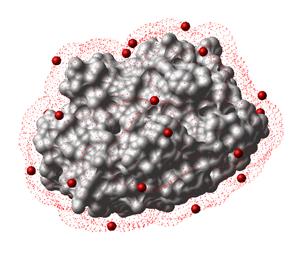
 Xyz( M_abs_xyz, R_3_6cell|obs )       → M_fract_xyz

 Xyz( M_fract_xyz, R_3_6cell|obs, cell ) → M_abs_xyz

Transforming absolute coordinates to fractional (i.e. the unit cell) coordinates and the inverse transformation. The cell parameters can be taken from an object or from the 3 or 6 cell parameters.

Example:

Xyz(Matrix({1. 2. 3.}),{10. 10. 10.}) # to fractionals

 #>M

 0.1 0.2 0.3

Xyz(Matrix({1. 2. 3.}),{10. 10. 10.} cell) # to absolute coordinates

 #>M

 10. 20. 30.

Applying crystallographic transformation

 Xyz( M_xyz, R_12abs_transformation [reverse|cell|transform] ) → M_xyz1_transformed

 Xyz( M_xyz, i_symm_transformation, s_sym_group, R3_cell|R_6_cell [cell|translate]) → M_xyz_transformed

 Xyz( M_xyz, i_symm_transformation, s_sym_group, R_6cell//R_3center ) → M_xyz_transformed

returns a new Nx3 coordinate matrix with the source coordinates transformed according to R_12abs_transformation or i_symm_transformation of the specified symmetry group.

If i_symm_transformation is greater than the number of symmetry operations in the specified symmetry group, the transformation goes to the 26 neighboring crystallographic cells. The central cell can be determined in three different ways:

• as {0. 0. 0.} (the default)
• automatically a mean point of M_xyz (option translate )
• as provided fixed point. These three coordinates can be appended to the 6 cell parameters, e.g. Cell(a_)//{10.,-2.,3.}

If option translate is provided or if {x,y,z} vector is appended to the 6-membered cell array The coordinates will be translated after the transformation to the cells around {x,y,z} .

Translation to the vicinity of automatically or statically defined center (option translate or {x,y,z} , accordingly) is also used by the transform command. The transform command does automated centering to the center of mass with the translate option or static with the translate={x,y,z} option.

Also see the makeBioMT macro.

Chemically matching a smiles string to a selection

 Xyz( as s_smiles ) → Xyz_match

Converting 3*N vector to a Nx3 coordinate matrix

 Xyz( R_3N_x1y1z1x2y2z3...> ) → <M_Nx3_xyz

Axis vectors of a crystallographic cell

 Xyz ( R_6cell axis )  → M_ABCvectors

returns three row-vectors A, B and C corresponding to the R_6cell parameters. The same vectors can be obtained as columns of the Augment(R_6 ) function. Example:

c6 = {10. 10. 10., 120. 120. 120.}
Xyz(c6,axis)[1] # A vector
Xyz(c6,axis)[2] # B vector
Xyz(c6,axis)[3] # C vector




---