|
Jul 1 2004
|
| Prev |
1.4 What can you do with ICM? (a program overview) | Next |
[ Graphics | Simulations | seqanalintro | modules ]
Let us go through the short overview of ICM applications.
[ funcprot | skinintro | nsr | ccr ]
The views include
- binding and active site surfaces with mapped properties
- automatic identification and views of cavities and open binding pockets
- electrostatic surfaces
|
|
|
The contour-buildup algorithm calculates the smooth and accurate
analytical molecular surface in seconds. This surface can be saved
as a geometrical object, saved as a vectorized postscript file.
|
|
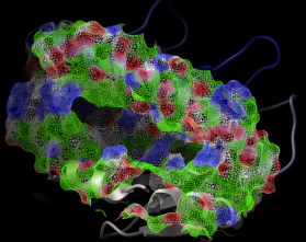
The skin is used in the REBEL algorithm to solve the Poisson
equation, as well as in the molecular surface analysis routines
(e.g. a projection of physical properties on the receptor surface ).
Also ICM can build and draw a solvent-accessible surface ( see surface)
and
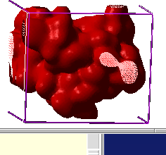
* a gaussian molecular density which can be contoured
at different levels and to generate different smooth molecular envelopes
and enclosed pockets and cavities:
 make map potential Box( a_ 3.)
 make grob m_atoms exact 0.5 solid
 display g_atoms smooth
|
|
PDB entry: 101d
ICM command:
nice "101d"
|
|
PDB entry: 4tna
ICM commands:
 nice "4tna"
 color ribbon a_N/* Count(Nof(a_N/*))
|
|
|
Simplified molecular representations are built automatically
(e.g. the protein-dna complex is shown with one command: nice "1dnk" ).
You can combine different types of molecular representations
with solid or wire geometrical objects.
|
Molecular representations include wire models, ball-and-stick models,
ribbons, space filling models, and skin representation.
[ pepfold | homomodels | loopmod | csym | dtp | dafltar | vlsintro | electrointro ]
|
Take a peptide sequence and predict its three-dimensional
structure. Of course, success is not guaranteed,
especially if the peptide is longer than about 25 residues
but some preliminary tests are encouraging.
|
You will also
get a movie of your peptide folding up. Just type the
peptide sequence in the _folding file and go ahead.
|
ICM has an excellent record in building accurate models by
homology. The procedure will build the framework, shake
up the side-chains and loops by global energy optimization.
You can also color the model by local reliability to identify
the potentially wrong parts of the model.
|
ICM also offers a fast and completely automated method to
build a model by homology and extract the best fitting loops
from a database of all known loops (see
build model and
montecarlo fast). It just takes a few seconds
to build a complete model by homology with loops.
|
ICM was used to design two new 7 residue loops and in both cases the designs
were successful. Moreover, the predicted conformations turned out to be exactly right
(accuracy of 0.5�) after the crystallographic structures of the designed proteins
were determined in Rik Wierenga's lab.
Use the _loop script to predict loop conformations and
calcEnergyStrain to identify the strained parts of the design.
|
|
ICM has a full set of commands and functions to generate
symmetry related molecules and generate "biological units".
|
Docking two proteins reliably is still an unsolved problem.
However, there has been a considerable progress. In some cases
(e.g. beta lactamase and its protein inhibitor) the ICM
docking procedure predicted the binding geometry correctly
based only on the global energy optimization.
ICM will generate a number of possible solutions using
both the explicit atom model of the receptor and the receptor
grid potential and
refine them by explicit global optimization of the surface side-chains.
Even though success is not guaranteed, the generated solutions
can be useful, especially if any additional information about the
binding is available.
As demonstrated in several recent papers, short flexible peptides
can be successfully docked ab initio to their receptors.
This method is a blend of the peptide folding with the
grid potentials representing the receptor. A similar method
can be applied to any chemical. A chemical can be built from
a 2D representation and optimized.
The "drugable" pockets can be predicted with an algorithm
based on the contiguous grid energy densities.
|
|
In virtual screening the flexible docking is applied to hundreds of thousands of individual ligands.
This version of docking is fast and requires an accurate relative binding
or ranking function to discriminate between the true ligands
and hundreds of thousands of potential false positives.
The ligand sampling and docking procedure is a combination of the
genuine internal coordinate docking methodology with a
sophisticated global optimization scheme.
|
Accurate and fast potentials and empirically adjusted scoring functions
have led to an efficient virtual screening methodology in
which ligands are fully and continuously flexible.
|
|
ICM incorporates a very fast and accurate boundary element solution of the
Poisson equation to find the electrostatic free energy of
a molecule in solution. This algorithm (abbreviated as REBEL)
can be used dynamically during conformational search.
The components of the electrostatic free
energy are used to calculate the binding energy and evaluate
the transfer energy between water and organic solvents.
ICM uses generalized Born approximation to
calculate the electrostatic solvation energy and its gradient
dynamically during local and global conformational searches.
|
The electrostatic potential can be projected on a molecular surface
for the identification of possible binding sites.
|
|
[ genomics | dotplotintro | seqalignintro | msaintro | evoltreeintro | zegaintro | plots3d ]
Handling gigabytes of genomic sequence, fast cross-comparison of
millions of sequences was another challenge solved in the ICM program.
ICM can identify a unique subset of millions of sequences,
assemble sequences from Unigene clusters into alignments (
SIM4 program is used a part of the procedure).
It looks like this:
Using the plotSeqDotMatrix macro:
 read sequence s_icmhome + "zincFing.seq"
 plotSeqDotMatrix 2drp_d 3znf_m \
 "Two z-finger peptide" "Human Enhancer Domain" 5 20
|
Here the color shows the local significance of the alignment. You can
change the method to calculate probability, color scheme and
residue comparison matrices and calculate it interactively or in batch.
|
|
Make a pairwise sequence alignment and evaluate the probability
that the two aligned sequences share the same structural fold.
The alignment is performed with the Needleman and Wunsch algorithm
modified to allow zero gap-end penalties (so called
ZEGA alignment). The ZEGA probability is a more sensitive
indicator of structural significance than the BLAST P-value.
The structural statistics was derived by
Abagyan and Batalov, 1997:
 read sequence s_icmhome + "sh3.seq"
 show Align(Fyn Spec)   # the probability will be shown
You can change residue comparison matrices, gap penalties and do many alignments in batch.
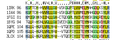
Read any number of sequences in fasta or swissprot formats and
automatically align the sequences, interactively or in a batch.
It will look like this:
# Consensus ...#.^.YD%..+~..-#~# K~-.#~##.~~..~WW.#.   ~~.~G%#P.
Fyn     ----VTLFVALYDYEARTEDDLSFHKGEKFQILNSSEGDWWEARSLTTGETGYIPS
Spec    DETGKELVLALYDYQEKSPREVTMKKGDILTLLNSTNKDWWKVE--VNDRQGFVP-
Eps8    KTQPKKYAKSKYDFVARNSSELSM-KDDVLELILDDRRQWWKVR---NSGDGFVPN

# nID 7 Lmin 56 ID 11.5 %
#MATGAP gonnet 2.4 0.15
ICM commands:
 read sequence s_icmhome + "sh3.seq"
 group sequences sh3
 align sh3
 show sh3
The gui version of ICM also has a multiple alignment viewer
with dynamic coloring according to conservation tables CONSENSUS and
CONSENSUSCOLOR. It will automatically show secondary structure and other features.
Relationships between sequences can be presented in three
forms:
- as evolutionary trees (ICM uses the neighbor-joining method for tree construction);
- as 2D distribution of sequences using the two main principal axes (use plot2Dseq macro);
- as 3D distribution. This can be analyzed in stereo using controls of
molecular graphics (use ds3D macro: ds3D Distance(alig) Name(alig) ).
|
|
Search your sequence (interactively or in batch) through any database and
generate a list of possible homologues which are sorted and evaluated by
probability of structural significance.
The ZEGA alignment (full dynamic programming with zero end gaps) is used
for each comparison and an empirical probability function described in JMB,1997 is used to assign a P-value to each hit.
This search may give you more homologues that a BLAST search!
The output may presented in a linked table form:
Table of hits
| NA1
| NA2
| ID
| SC
| pP
| DE
| |
| Fyn
| 1nyf_mNo
| 100.
| 62.81
| 20.94
| fyn
|
| ...
| lines skipped
| ...
| ...
| ...
| ...
|
| Eps8
| 1tud_m17
| 21.
| 17.04
| 4.17
| alpha-spectrin
|
| Eps8
| 1fyn_a23
| 22.6
| 17.02
| 4.16
| phosphotransferase fyn
|
| Eps8
| 1efn_a25
| 22.
| 16.64
| 4.11
| fyn tyrosine kinase
|
| Eps8
| 1hsq_mNo
| 24.2
| 16.87
| 4.1
| phospholipase c-gamma (sh3 domain)
|
Take a matrix and represent it in 3D in a variety of forms.
View it in stereo, color, label, transform with the mouse.
Example:
 read matrix s_icmhome + "def"
 make grob def solid color
 display
|
|
|
ICM is distributed in the following packages:
- ICM-main
- ICM-bioinfo (sequence analysis)
- ICM-REBEL (electrostatics)
- ICM-docking (includes cheminformatics)
- ICM-pro (includes the above four modules)
- ICM-homology (fast homology building and database loop searches in addition to ICM-pro)
- ICM-VLS (virtual ligand screening, includes ICM-pro)
The modules have the following features:
!_ ICM-main
- shell for molecules, numbers, strings, vectors, matrices, tables, sequences, alignments, profiles, maps
- ICM-language and macros
- graphics, stereo
- imaging and vectorized postscript
- animation and movies
- mathematics, statistics, plotting
- presentation of the results in html format
- user-defined and automated interpretation of web links
- HTML-form-output interpretation
- pairwise and multiple sequence alignments, evolutionary trees, clustering
- secondary structure prediction and assignment, property profiles, pattern searching
- superpositions, structural alignment, Ramachandran plots
- protein quality check
- analytical molecular surface
- calculations of surface areas and volumes
- cavity analysis
- symmetry operations, access to 230 space groups
- database fragment search
- identification of common substructures in PDB
- read pdb, mol2, csd, build from sequence
- energy, solvation, MIMEL, side-chain entropies, soft van der Waals, tethers, distance and angular restraints
- local minimization
- ab initio peptide structure prediction by the Biased Probability Monte Carlo method
- loop simulations
- side-chain placement
!_ ICM-REBEL (electrostatics)
- electrostatic free energy calculated by the boundary element method
- coloring molecular surface by electrostatic potential
- binding energy (electrostatic solvation component)
- maps of electrostatic potential and its isopotential contours
!_ ICM-docking and chemistry
- indexing of chemical databases in SD, mol2 and csd format
- searching and extracting from the indexed databases
- fast grid potentials
- scripts for flexible ligand docking
- scripts for protein-protein docking
- 2D (SMILES) to 3D conversion, type and charge assignment,
mmff geometry optimization, low-energy rotamer generation
- refinement in full atom representation
!_ ICM-bioinformatics
- fast comparison and redundancy removal of millions of genomic or protein sequences
- multiple EST clustering, alignment and consensus derivation
- database indexing and manipulations
- functions to evaluate sequence-structure similarity
- scripts to recognize remote similarities in the protein sequence and PDB databases
- search a pattern through a database
- searching profiles and patterns from the Prosite database through a sequence
- HTML representation of the search results with interpretation of links
- interactive editor of sequence-structure alignment
- automated building of models by homology with loop sampling and side-chain placement (fast homology model building combined with the database loop search is a separate module which is ICM Homology).
!_ ICM-Homology
- sequence-structure alignment (threading)
- ultra-fast automated homology model building with a database loop search
- loop modeling and refinement, side-chain placement
- surface analysis
As a method for structure prediction, ICM
offers a new efficient way of global energy optimization and versatile modeling
operations on arbitrarily fixed multimolecular systems.
It is aimed at predicting large structural rearrangements in biopolymers.
The ICM-method uses a generalized description of biomolecular structures in which bond lengths,
bond angles, torsion and phase angles are considered as independent variables.
Any subset of those variables can be fixed. Rigid bodies formed after
exclusion of some variables (i.e. all bond lengths, bond angles and
phase angles, or all the variables in a protein domain, etc.) can be
treated efficiently in energy calculations, since no interactions within
a rigid body are calculated. Analytical energy derivatives are calculated
to allow fast local minimization. To allow large scale conformational
sampling and powerful molecular manipulations ICM employs a family of
new global optimization techniques such as:
Biased Probability Monte Carlo ( Abagyan and Totrov, 1994),
pseudo-Brownian docking method ( Abagyan, Totrov and Kuznetsov, 1994)
and local deformation loop movements Abagyan and Mazur, 1989).
A set of ECEPP/3 energy terms is complemented with the parameters for
rare atoms and atom types, as well as the solvation energy terms,
electrostatic polarization energy
and side-chain entropic effects ( Abagyan and Totrov, 1994),
making the total calculated energy a more realistic approximation
of the true free energy.
The MMFF94 force field has also been implemented.
Powerful molecular graphics, the ICM-command language,
and a set of structure manipulation tools and penalty functions (such as
multidimensional variable restraints, tethers, distance restraints) allow
the user to address a wide variety of problems concerning biomolecular
structures.
|