| Prev | 2.20 Commands | Next |
[ addtable | alias | align | appendcolumn | assign | break | build | call | center | clear | color | compare | compress | connect | continue | convert | copy | crypt | delete | display | elseif | endfor | endif | endmacro | edit | endwhile | exit | find | fix | for | fork | fprintf | global | goto | group | _gui | help | history | if | keep | learn | linkvariable | linkalignment | list | listbinary | listdatabase | load | macro | make | minimize | menu | modify | montecarlo | move | pause | _plot | plotarea | print | printf | printimage | quit | randomize | read | rename | renameobject | return | rotate | set | show | sort | split | sprintf | store | ssearch | strip | superimpose | sys | then | transform | translate | undisplay | unfix | wait | web | webtable | while | write ]
2.20.1 add/insert table rows. | [Top] |
add/insert rows to table T_1 after position i_prevRow ( 0 if you need to insert the first line). If the 3rd argument is not provided, adds an empty row. The row_selection can contain rows from the same table or from a different table with a matching column structure. In the latter case, the columns can be named differently, but the number of columns and their types must match (see example below). The defaults for an empty line are empty string or zero value for strings or numbers, respectively.
Examples:
group table t {1 2 3} "a" {"b","d","e"} "b"
show t
 #>T t
 #>-a-----------b----------
    1           b
    2           d
    3           e

add t 0 # insert empty line before 1st
show t
 #>T t
 #>-a-----------b----------
    0           ""
    1           b
    2           d
    3           e

group table t {1 2 3} "a" {"b","d","e"} "b" # redo the table
add t 2 t[1]  # insert a duplicate of 1st row after the 2nd
 #>T t
 #>-a-----------b----------
    1           b
    2           d
    1           b
    3           e

group table t {1 2 3}  "a"  {"b","d","e"} "b"  # redo the table
group table tt {1 2 3} "aa" {"b","d","e"} "bb" # another table
# column names are different, but the structure is the same
add t 2 tt[1:2]  # or add t 2 tt.aa<3
show t
 #>T t
 #>-a-----------b----------
    1           b
    2           d
    1           b
    2           d
    3           e
2.20.2 alias | [Top] |
create alias
alias delete abbreviation
delete alias
It is important that the abbreviation is not used in the ICM-shell. The same names can not be given later to ICM-shell objects.
Alias may contain arguments $0, $1, $2, etc. ICM-shell will pick space-separated words following the alias name and substitute $1, $2, etc. arguments by the specified argument. $0 stands for all the arguments after the alias name.
Examples:
 alias seq sequence                    # seq will invoke sequence
 alias delete seq                      # delete alias name seq
 alias dsb display a_//ca,c,n          # abbreviate several words to
                                       # reduce typing efforts
                                       # aliases with arguments
 alias NORM ($1-Mean($1))/Rmsd($1)
 show NORM {6,7,8,4,6,5,6,7,5,6}       # make sure there is no space
2.20.3 align | [Top] |
[ alignnumber | alignsequence | alignfragments | align3D | align3Dheavy ]
2.20.3.1 align number: renumber residues sequentially | [Top] |
align number ms_chainsToBeRenumbered [ i_firstNumber ]
renumber selected residues, or residues in selected molecules or objects sequentially in all of them from starting one or the specified first number. May be useful to deal with messy numbering in some pdb-files. Example:
 read pdb "1crn"
 align number a_1            # renumber all res. 1 to N
 align number a_1/10:20 101  # just the selected residues from 101
 align number a_1       101  # renumber all res. 101 to 100+N
align number ms_chainsToBeRenumbered seq_master [ i_offset ] renumber the residues of the selected molecule according to seq_master master sequence which is aligned to the sequence of the selected chain. The alignment (pairwise or multiple) need to be linked to the molecule/chain and both the chain sequence and the master sequence need to be covered by the alignment. The molecular sequence can be generated with the make sequence [ ms_chainsToBeRenumbered ] command. The can be either aligned anew the the master sequence with the Alignfunction or appended to a multiple sequence alignment using alignment projection.
This command may be useful in cases in which a structural model does not represent the entire sequence because of omitted loops, N- and C- termini, while you still want to keep the numbering according to the full master sequence. You might want to use the command also on models by homology generated with the build model command.
Example:
 seqmaster = Sequence("ACDEFGHIKLMNPQRST")
 buildpep             "--DEFGH-----PQRST"  # dashes are skipped
 make sequence a_1 name="seqmodel"         # sequence is auto-linked
 a = Align(seqmodel,seqmaster)             # linked alignment
 align number a_1 seqmaster
 # Info> residues of a_def.m renumbered by sequence 'seqmaster' from alignment 'a'
 display residue label
2.20.3.2 align: ICM multiple alignment algorithm | [Top] |
make a multiple alignment of specified sequences a sequence group resulting from the group sequence s_groupName command. For pairwise alignment use the Align seq1 seq2 ) function. The algorithm includes the following steps (inspired by corridor discussions with Des Higgins, Toby Gibson and Julie Thompson ):
- align all sequence pairs with the ICM ZEGA algorithm, and calculate pairwise distances between each pair of aligned sequence with the Dayhoff formula, e.g. the distance between two identical sequences will be 0. , while the distance between two 30% different sequences will be around 0.5. The distance goes to an arbitrary number of 10. for completely unrelated sequences. The distance matrix Dij can later be extracted from the alignment with the Distance( ali_ ) function.
- build an evolutionary tree from Dij with the "neighbor-joining algorithm" of Saitou, N., Nei, M. (1987) to determine the order of the alignment and calculate relative weights of sequences and profiles from the branch lengths. The tree will be saved in the file defined by the tree option (aligTree.eps file by default). The so-called Newick tree description string will be saved in s_out .
- traverse the tree from top to bottom, aligning the closest sequences, sequence and profile or two profiles. After each Needleman and Wunsch alignment, build the profile.
- generate the final neighbor-joining evolutionary tree and write the PostScript file with the tree to disk.
Examples:
   read sequences s_icmhome+"zincFinger"
   list sequences               # see them, then ...
   group sequence alZnFing      # group them, then ...
   align alZnFing               # align them, then ...
   unix gs aligTree.eps         # ... evolutionary tree ready
                                # (gs is a PostScript previewer)
2.20.3.3 EST,DNA alignment and assembly | [Top] |
[ sim4 ]
align new ali_sequenceGroup [ seq_seed ]multiple alignment of ESTs and genomic DNA and consensus derivation. This command uses the external the sim4 program to generate pairwise alignments between expressed DNA sequence and a genomic sequence. The program can be downloaded from the http://globin.cse.psu.edu/globin/html/docs/sim4.html site.
The procedure has the following steps:
The result of this command is best displayed with the show color ali_ command. |
|
An example:
 read sequence "http://www.ncbi.nlm.nih.gov/UniGene/" + \
     "download.cgi?ID=5198&ORG=HsLINE=1</tt> #
 read sequence "../Hs5198"
 group sequence unique u # squeeze out obvious redundancies and form group 'u'
 align new u             # form multiple alignment and build consensus
 show color u
See also:
- filtering, group sequence unique=".."
- Trans ()
- show [color] ali_
2.20.3.4 align two molecules by their backbone topology | [Top] |
| This command finds the residue alignment (or residue-to-residue correspondence) for two arbitrary molecules having superimposable parts of the backbone conformations. The structural alignment identification and optimal superposition is primarily based on the C-alpha-atom coordinates, but the sequence information can be added with a certain weight (the default value of r_seqWeight is 0.5 which was found optimal on a benchmark). The structural alignment algorithm is based on the ZEGA (zero-end-gap-alignment) dynamic programming procedure in which substitution scores for each i,j-pair of residues contain two terms: |
|
- structural similarity in a i_windowSize window between two fragments surrounding residues i and j, respectively. This similarity is calculated as local Rmsd of the residue label atoms (these atoms are C-alpha atoms by default but can be reset to other atoms with the set label command, e.g. set label a_*.//cb ). If the option distance is specified the deviation of the interatomic distances between equivalent pairs of atoms (so called distance rmsd ) is calculated instead of a more traditional root-mean square deviation between atom coordinates of equivalent atoms. The latter method is less accurate but an order of magnitude faster.
- sequence similarity (if r_seqWeight > 0.). Average local sequence alignment score in the i_windowSize window is calculated for i,j-centered pair of fragments. In this sense this sequence similarity is different from the one used in pure sequence alignment (see the Alignfunction), in which just the i,j residue pair is evaluated. The default value of r_seqWeight of 0.5 is rather mild (about a half of the structural signal).
The output:
- ali_out contains structural alignment (if sequences linked to the molecules do not exist, they will be created on the fly). The alignment can be further edited with the interactive alignment alignment editor.
- as_out contains the residue selection of the aligned residues in the first molecule
- as2_out contains the residue selection of the aligned residues in the second molecule
- M_out , the matrix of local structural/sequence similarity in a window is retained and can be visualized by:
make grob color 10.*M_out name="g_mat # x,y,z scales
display g_mat
# or
plot area M_out display grid link
See also:
- Align seq_1 seq_2 distance|superimpose ). This function creates the first unrefined structural alignment as described above.
- find alignment which refines initial structural alignment.
  a = Align(... superimpose )  # superposition/RMSD based local str. alignment
  a = Align(... distance    )  # distance RMSD based local str. alignment

  find a superimpose 4.0 0.5
Example:
  read object s_xpdbDir + "/1brl.b/"
  read object s_xpdbDir+"/1nfp"
  rm a_*.!A
  display a_*.//ca,c,n
  color molecule a_*.
  align a_2.1 a_1.1
  center
  show String(as_out) String(as2_out)
  color red as_out
  color blue as2_out
  show ali_out
2.20.3.5 align heavy command for multiple alternative structural alignments. | [Top] |
[ appendaliseq ]
align heavy rs_1 rs_2 [ r_rmsd ] [ i_windowSize [ i_minFragment]] [ r_elongationWeight]This method, as opposed to the default align ms_1 ms_2 generates many possible solutions and does not depend on sequential order of the secondary structure elements. However, it leads to a combinatorial explosion and is intrinsically less stable computationally, and generally requires more time. The command finds the optimal 3D superposition between two arbitrary molecules/fragments (two residue selections rs_1 and rs_2 ).
The procedure generates structural fragments of certain initial length and superimposes all of them to calculate the structural similarity distance. Then the "islands" of similarity are merged into larger pieces. This process is controlled by the following arguments: i_windowSize is the residue length of structural fragments for the initial fragment superposition. Fragment pairs with the rms deviation less than r_rmsd are then combined, giving composite solutions of total residue length larger than i_minFragment. Acception or rejection of the composite solutions is governed by the following score (the smaller, the better)
score = rmsd - (1.37 + Sqrt(1.16 * length - 15.1)), length >= 14
If length > 14 , we use linear extrapolation of the score dependence:
score = rmsd - (1.37 + 1.068*(length-13))
The score is required to be less than r_rmsd. Practically, for longer fragments one can find much larger RMS deviations according to the length correction of the score.
Defaults:
- r_rmsd = 1. A
- i_windowSize = 15 residues
- i_minFragment = i_windowSize
- r_elongationWeight=0.1
See also: How to optimally superimpose without the residue alignment
Example:
read pdb "4fxc" read pdb "1ubq" display a_*.//ca,c,n color molecule a_*. align heavy a_1.1 a_2.1 12 1.5 .1 center load solution 2 # load the second best solution color red as_out color blue as2_out for i=1,10 load solution i color molecule a_*. color red as_out color blue as2_out pause # rotate and hit 'return' endforNote. Increase i_minFragment parameter (12 in the above example) to something like 20 if the program hangs for too long. Interrupt execution with the ICM-interrupt (Ctrl \) if you want only the top solutions.
: append
appends sequences to a sequence group. This may be required if you formed a sequence group for future alignment or filtering/compression and you want to append additional sequences to it. E.g.
read sequence group "bunch.seq" name="xx" # group xx is formed
append xx my_seq  # appending your sequence to xx
group xx unique   # filter out identical ones
align xx
2.20.4 append two tables by share column | [Top] |
Append rows of table t2 to table t1 by rows corresponding to unique column t2.B . The t1.A column values do not need to be unique.
group table people {"J","C","M"} "p" {"MS","MS","MS"} "orgid"
group table orgs  {"MS"} "id" {"Molsoft"} "name"
append people.orgid orgs.id
people
 #>T people
 #>-p-----------orgid-------name-------
    J           MS          Molsoft
    C           MS          Molsoft
    M           MS          Molsoft
2.20.5 assign | [Top] |
[ assignsstructure | assignsstructuresegment ]
2.20.5.1 assign sstructure: derive secondary structure from a pattern of hydrogen bonds | [Top] |
Manual assignment of a desired secondary structure annotation to a residue fragment
assign specified secondary structure to the selected residues rs_ , e.g.
 read pdb "1est"
 assign sstructure a_/* "_"  # make everything look like a coil
 cool a_
 assign sstructure a_/1:10 "HHHH_EEEEE"
 cool a_
|
This command does not change the geometry of the model, it only formally assigns secondary structure symbols to residues. Note: to change the conformation of the selected residue fragment, according to a desired secondary string, use the ICM -object and the set command applied to both sequences and molecular objects. |
Automated derivation and assignment of secondary structure from atomic coordinates
assign sstructure rs_
If the secondary structure string is not specified, apply ICM modification of the DSSP algorithm of automatic secondary structure assignment (Kabsch and Sander, 1983) based on the observed pattern of hydrogen bonds in a three dimensional structure.
The DSSP algorithm in its original form overassigns the helical regions. For example, in the structure of T4 lysozyme (PDB code 103l ) DSSP assigns to one helix the whole region a_/93:112 which actually consists of two helices a_/93:105 and a_/108:112 forming a sharp angle of 64 degrees. ICM employs a modified algorithm which patches the above problem of the original DSSP algorithm. Assigned secondary structure types are the following: "H" - alpha helix, "G" - 3/10 helix, "I" - pi helix, "E" - beta strand, "B" - beta-bridge, "_" or "C" - coil.
Examples:
 nice "1est"       # notice that many loops look like beta-strands
 assign sstructure # now the problem is fixed
 cool a_
See the set rs_ s_SecStructPattern command to actually set new phi, psi angles to a peptide backbone according to the string of secondary structure.
2.20.5.2 assign sstructure segment | [Top] |
create simplified description of protein topology (referred to as segment representation). Segments shorter than segMinLength are ignored. The current object is the default.
See also show segment, ribbonStyle, display ribbon.
2.20.6 break | [Top] |
Examples:
   for i = 1, 8
     print "Now i = ", i, "and it goes up"
     if (i == 4) then
       print "... but at i=4 it breaks, Ouch!"
       break
     endif
  endfor
See also
goto .
2.20.7 build | [Top] |
[ buildseq | buildmodel | buildloop | buildstring | buildhydrogen ]
The build family of functions allows to create molecular objects- from sequence file ( build s_seqfile )
- from sequence string ( build string)
- from a linear chemical notation ( build smiles )
- from a sequence and a template by homology ( build model )
2.20.7.1 build from sequence file | [Top] |
reads s_IcmSeqFileName.se ICM-sequence file and builds an ICM molecular object. This sequence file is different from a simple sequence file and contains three (sometimes four) character residue names defined in the icm.res residue library file (try show residue types to see the list). Use macro buildpep if you want to build an object from a string with one letter coded sequences or a named sequence (see the build string command below). The buildpep macro also allows to easily create several molecules by using a semicolon ; separator. To get a D-amino acid instead of L-ones simply use D as a prefix: Dala Darg. Specify N- or C-terminal modifiers directly in the file if needed. The build command will create them in some default conformation (extended backbone with different molecules oriented around the origin as a bunch of flowers). Several molecules can be specified in the ICM sequence file.
Residue names can contain numbers (i.e. 4me ). However, the residue numbers with a modification character, such as 44a, 44b should contain a slash before the modification character (i.e. 44/a , 44/b ). An example in which we create a sequence of residues ala and 4me with numbers 2a and 2b, respectively: "se 2a ala 2b 4me".
Option library= lets you temporarily switch the library file. It can also be done by redefining the LIBRARY.res array of the LIBRARY table.
Option delete temporarily sets the l_confirm flag to no and the old object with the same name gets overwritten.
Examples:
 build          # def.se file
 build "alpha"  # alpha.se file
 build "wierd" library="mod.res"  # get residues from mod.res
#
 LIBRARY.res = {"icm","./myres"}
 build "a"
Use a convenient macro buildpep to build one or several-chain peptides with one- or three- letter code. E.g.
 buildpep "ASFGDH;FFF"  # two molecules
 buildpep "ala his trp" # one chain of three residues
2.20.7.2 build model by homology | [Top] |
build a comparative model (homology model) of the input sequences based on the similarity to the given molecular objects. The margin arguments:
| name | default | description |
|---|---|---|
| i_maxLoopLength 999 longer loops are dropped | ||
| i_maxNterm 1 the maximal length of the N-terminal model sequence which extends beyond the template | ||
| i_maxCterm 1 the maximal length of the C-terminal model sequence which extends beyond the template | ||
| i_expandGaps 1 additional widening of the gaps in the alignment. End gaps are not expanded |
-
Possible modes:
- simple one-to-one mode: build model seq_1 [ms_1] [ali_1]
- N sequences - N corresponding molecules: build model seq_1 seq_2 .. seq_N ms_1,2,..N
Example:
 l_autoLink = yes
 read pdb "x"
 read alignment "sx"
 build model ly6 a_
 ribbonColorStyle = "alignment" # grey-gaps, magenta-insertions
 display ribbon
#
 read pdb "2ins"  # multichain
 read sequence unix cat
> a
GIVEQCCASV CSLYQLENYC N
> b
VNQHLCGSHL VEALYLVCGE RGFFYTPKA
> c
GIVEQCCASV CSLYQLENYC N
> d
VNQHLCGSHL VEALYLVCGE RGFFYTPKA
^D
 build model  a b c d a_1.
# Now optimize the side chains
 selectMinGrad = 1.5
 set vrestraint a_/*
 montecarlo fast v_/!I/x*
# !I means residues which are not Identical to their template residues
# use  refineModel  to energetically optimize the model
!_ The algorithm performs the following steps:
Alignment adjustment: modifies the alignment according to i_expandGaps, and prepare a sequence with the ends and the long loops truncated according to the alignment and the { i_maxLoopLength , i_maxNterm , i_maxCterm } parameters.
Building a straight polypeptide from the model sequence: builds a full-atom polypeptide chain for this new sequence. The residues in your model are numbered according to the template and all the inserted loops residues are indexed with 'a','b', etc. E.g. the numbering may look like this: 200,201,203,204,204a,204b,204c,205 ... This numbering allows one to follow more easily the correspondence between the template and the model. If you do not like this numbering scheme, just use the
align number a_/*command and the model residues will be renumbered from 1 to the number of residues.
Backbone topology transfer: inherits the backbone conformation from the aligned (but not necessarily identical) parts of the known template
Identical side-chain building: inherits conformations of sidechains identical to their template in the alignment
Non-identical side-chain placement: assigns the most likely rotamer to the side chains not identical in alignment. If you want to do more than that apply:
set vrestraint a_/*  # assigns the rotamer probabilities
montecarlo fast v_/Cx/x* # x* selects for all chi (xi) angles
You can also manually re-optimize any side chains either interactively (right-mouse click on a residue atom, then select Shake Amino-Acid Side-Chain) or from a script, e.g. for residue 14:
set vrestraint a_/*  # assigns the rotamer probabilities
montecarlo v_/14/x*
ssearch v_/14/x*     # systematic conformational search for the 14-th sidechain
!_ Loop searches: searches the icm.lps which may contain entire PDB-database for suitable loops with matching loop ends and as close loop sequence as possible, inserts them into the model and modifies the side-chains according to the model sequence.
The loop file can be easily customized, updated and rebuilt with the write model [append] command in a loop over protein structures. To use your custom loop file, redefine the LIBRARY.lpsvariable.
!_ Loop refinement and storing alternatives: adjusts the best loops found and keeps a stack of loop alternatives which can later be tested (see the Homology gui-menu)
!_ The output
The build model command returns the following variables:
LoopTable master table containing list of all the loops, their conformation in alphanumeric code, a measure of the deviation of the database loop ends and the model attachment sites, the loop length and the numerical conformation type (not really important). E.g.
#>T LoopTable
#>-1_Loop------2_Conf------3_Rmsd------4_Nof-------5_Type-----
   a_ly6.a/7:10 31R21       0.1         11          1
   a_ly6.a/60:63 1RRR32      0.1         8           1
   a_ly6.a/43:46 211331RRRR  0.240658    4           1
Individual loop tables
Tables called LOOP1 , LOOP2 , etc. for each inserted loop. The tables contain the coded conformational string, relative energy, the position of the offset in the structure database file ( offset ) to be able to extract this loop again, and the rmsd of the loop ends. Example:
icm/ly6> LOOP1
#>T LOOP1
#>-Conf--------energy------offset------rmsd-------
   31R21       0.          3623594     0.092104
   31RR2       1.519275    3427772     0.083372
   R1121       1.612712    3750108     0.097777
   R1R32       1.639177    1529882     0.087113
   R1RR2       1.880638    3806768     0.079335
   31R32       3.714823    4561270     0.053853
   R3RR2       4.531406    4003324     0.042881
!_ Writing and restoring the tethers You can write both template and the model and the tethers between them to files (see section write tethers .
!_ Trouble shooting build model may crash. A possible reason of the crash is that the pdb file is not correctly parsed due to formatting errors. Many pdb files still have formatting errors, especially those which are generated by other programs or prepared manually. In this case the read pdb command is trying to interpret the field shifts and, as with any guess work, frequently gets it wrong. For example, try 2ins and you will see that the atom or residue names are shifted. To fix the problem, try to use the exact option of the read pdb command.
2.20.7.3 build loop to a model by homology | [Top] |
[ buildsmiles ]
build loop rs_fragmentsrebuild specified loop based in a PDB-database search (see build model ).
An example:
 read object s_icmhome+"crn"
 build loop a_/20:26  # rebuild this loop
: build [ smiles | sln ]
|
create an ICM-object from the smiles-stringor sln-string respectively. Set l_readMolArom to no if you do not want to assign aromatic rings from a pattern of single and double bonds (and formal charge and bond symmetrization for CO2, SO2, NO2or3, PO3 ) upon building. To suppress suppress the symmetrization and consequential charging of CO2, set the l_neutralAcids flag to yes . |
Examples:
  build smiles "CCO"   # ethanol

  build smiles "Oc(cc1cc2)ccc1cc2N"

  build smiles "Oc(cc1cc2)cc(ccc3)c1c3c2"

                # dicoronene
  build smiles "c1c2ccc3ccc4c5c6c(ccc7c6c(c2c35)c2c1c1c3c5c6c"+\
               "(c1)ccc1c6c6c(cc1)ccc1ccc(c5c61)cc3c2c7)cc4"

                # NAD
  build smiles "[O-]P(=O)(OCC1OC(C(O)C1O)N1C=2N=CN=C(N)C=2N=C1)"+\
               "OP(=O)([O-])OCC1OC(C(O)C1O)N=1C=CC=C(C=1)C(=O)N"

                # Hexabenzo(bc,ef,hi,kl,no,qr)coronene
  build smiles "c1c2c3c4c(ccc3)c3c5c(c6c7c(ccc6)c6c8c(ccc6)c6c9"+\
               "c(ccc6)c(cc1)c2c1c9c8c7c5c41)ccc3"

                # rubrene
  build smiles "c1c2c(c3ccccc3)c3c(c(c4ccccc4)c4c(cccc4)c3c3ccccc3)"+\
               "c(c2ccc1)c1ccccc1"
Usually the build smiles command is not sufficient. The molecule needs
to be optimized in the mmff force field and several conformations
need to be sampled.
The quick way of doing it is shown below.
 build smiles "CC=1C(=O)C=CC(C=1)=O"
 strip a_
 build hydrogen
 set type mmff
 set charge mmff
 convert
 read library mmff
 tolGrad = 0.001
 ffMethod = "mmff"
 minimize cartesian
A more rigorous way of doing the conversion is done with this macro:
macro scan2Dto3Dconvert
  oldGrad = tolGrad
  tolGrad = 0.0001
  ffMethod = "mmff"
  vwMethod = "soft"
  unfix V_//a* & !V_//avt*
  v =  Value( v_//a* & !V_//avt* )
  m = Matrix( Nof( v) 2 )
  m[?,1] = v
  m[?,2] = Rarray( Nof( v) 170. )
  v = Min (Transpose( m ) )
  set v_//a* & !V_//avt* v
  delete m v
  fix V_//a* & !V_//avt*
  delete stack
  store conf 1
  for i=2,5
    load conf 1
    randomize a_// 0.03
    randomize v_//
    store conf i
  endfor
  minimize stack "vw,14,to,hb"
  errorAction = "none" # avoid crashing on cartesian min.
  minimize cartesian stack 3000 "vw,14,to,hb,bb,bs,af"
  if(!Error()) then
    load conf 0
  else
    load conf 1 # try to restore a good conformation
  endif
  vwMethod = "exact"
  minimize cartesian 3000 "vw,14,to,hb,el,bb,bs,af"
  if(Error()) print "ERROR> 2Dto3D failed"
  errorAction = "break"
  delete stack
  tolGrad = oldGrad
  randomize a_//* 0.01
endmacro
See also the Smiles function and the find molecule s_Smiles1 S_Smiles2 command to find a substructure
2.20.7.4 build object from string | [Top] |
create an ICM-object from a s_IcmSequence string (see the build command above). To get a D-amino acid instead of L-ones simply use D as a prefix: Dala Darg. Specify N- or C-terminal modifiers directly in the file if needed. The build command will create them in some default conformation.
Option delete temporarily sets the l_confirm flag to no and the old object with the same name gets overwritten.
Examples:
   build string "se nh3+ ala his coo-" name="pep"  # one peptide named a_pep.
   build string "ml a \nse nh3+ his coo- \nml b \nse trp" # molecules a and b
   build string IcmSequence("GHFDSFSDRT","nter","cooh") # translate and add termini
#
# Using alias  BS   build string "se $0"
   BS ala his trp
#
# Using alias  BSS  build string IcmSequence( $0 )
   BSS "SFGDFAGSFG"   # quoted one-letter code string
   read sequence "GTPA_HUMAN.seq"
   BSS GTPA_HUMAN     # sequence name
2.20.7.5 build hydrogens according to topology and formal charges. | [Top] |
add hydrogens to the specified heavy atoms according to their type and formal charge. All heavy atoms of the current object are used by default. If your have hydrogens already and their configuration is wrong, you can delete them with the delete hydrogen command. The number of hydrogens may be enforced if the optional i_forcedNofHydrogens argument is specified. See also the set bond type command.
Examples:
   read mol2 s_icmhome+ "ex_mol2"  # several small molecules
   display a_4.
   build hydrogen a_4.  # added and displayed
2.20.8 call icm script | [Top] |
invokes and executes an ICM-script file. End the script with the quit command, unless you want to continue to work interactively, or use it in other script.
Option only allows you to suppress opening the script file if the call command is inside a block which is not executed. By default the script file is opened and loaded into the ICM history stack anyway, but the commands from the file are not executed.
The absolute path of the script can be return by the Path ( last ) function.
Calling scripts inside conditional expressions.
Examples:
   call _startup             # execute commands from _startup file


   if Version() !~ "* R *" goto skip:    # Rebel is not licensed
     call _rebel only  # only means do not read _rebel if skipped.
skip:
2.20.9 center | [Top] |
centers and zooms the screen on selected atoms as_ or graphics objects. Default objects: all existing atoms and graphics objects. The r_margin argument is given in Angstrom units and can be used to set a relative size of the selection and the frame. Normally all dimensions of the molecule/grob are taken into account, so that the molecule can be rotated without changing scale.
Options:
- only : do not rescale, translate only, i.e. move the selected atoms to the center of the graphics window
- static : scale only according to the visible X-Y dimensions and the margin. Do not take the Z-dimension into account in the size calculation as if you do not intend to rotate objects. That implies an assumption that the orientation of molecules/grobs/maps will not be changed.
Examples:
   nice "1est"
   center
   center Sphere ( a_/15:18 )
   center a_/1:2 only  # keep the scale

   read grob s_icmhome+"beethoven" # a genius
   display g_beethoven smooth
   center g_beethoven static   # 10 A margin
2.20.10 clear | [Top] |
clear selection clear the graphical selection as_graph
clear error clear all error and warning bits previously set by ICM. See also Error ( i_code )
2.20.11 color family of commands | [Top] |
[ colormolgrob | colorbackground | colorbyalignment | colorcursor | colorgrob | colorlabel | colormap | colormolecule | colorribbon | colorvolume ]
The color command colors different shell objects, their parts, or different graphical representations with by colors specified in various ways.2.20.11.1 color: main command | [Top] |
color [ { as_ | g_grobName } ] [ wire | hbond | cpk | ball | stick | xstick | surface | skin | site | ribbon [base]] [ color_specification ]
The color can be specified as
color_name | s_ColorName | color[i_index] | i_Color | r_Color | I_Color | R_Color | rgbr=R_3rgb [ window = R_MinMax ]
color selected atoms ( as_ ) or graphics object(s) according to specified color. The window={minValue,maxValue} option allows to provide a range for color mapping. Example:
color ribbon a_/ Bfactor(a_/ simple) window=-0.5//2.This command will clamp Bfactor(a_/ simple) values which are normally around zero, but may range from large negative values to large values, to the [-0.5,2.] range.
The defaults:
- objects: the current object ( a_ ) only (to color all objects, use a_*. )
- graphic representation: all except ribbon. To color ribbon specify use color ribbon
- color: the default coloring (atoms - by atom type, which can be changed in the icm.clr file; ribbon - by secondary structure )
 nice "1crn"
 display       # also displays wire
 color         # all except ribbon colored by atom type
 color ribbon  # only ribbon of a_ by secondary structure type
 color ribbon red         # only ribbon as specified
 color a_1,2. ribbon red  # only ribbon as specified
color_name. Color may be just a word (such as black, white, grey, blue, red, yellow, green, orange, magenta, ... ) or string (as "green"), or integer (convenient for automatic coloring within ICM loops), or integer array, or real array (to color according to a certain property, as electric charge or Bfactor). Default: color by atom type; in ribbon representation by secondary structure type.
In DNA and RNA ribbons, bases can be colored separately (e.g. color ribbon base a_1/* white ), the default coloring being A-red, C-cyan, G-blue, T or U-gold. Colors themselves and all the defaults may be changed in the icm.clr file. Different color specifications with examples:
color red unquoted color name
color "red" quoted color name or a string variable
color color[4] use color number 4 from the list of "named" colors (first section of the icm.clr file). You can show the colors with their numbers by the show color command and their total number is accessible via the Nof( color) function. This mode is useful if you need to color selected elements with contrasting colors rather than with a smooth spectrum.
Example:
   display a__crn.             # load and display molecule
   show colors
   color a_/1:5/* color[89]
   for i=1,Nof(a_/*)
    color a_/$i color[i]       # gay coloring
   endfor
color 3 (integer) color number from the "rainbow" section of the icm.clr file. Currently there are 128 colors (i=0,127) in this section and they form a smooth transition from blue to red via white (not really a rainbow). You may change the "rainbow" colors in the icm.clr file. Number 128 becomes blue again. Execute these lines to see how it goes:
   display "Colors"
   for i=1,255
     color background i
     print i
   endfor
color 4.5 (real) similar to the previous type. The color is interpolated. 4.5 will be the average between the "rainbow color" 4 and "rainbow color" 5.
color selection 1,3,5 or color selection 1.,3.,5. color each element of the selection by I_Color or R_Color. The scale is determined by the minimal and the maximal elements of the array, independently of the array length. First the numbers in the array are scaled so that its minimum corresponds to the first color in the "rainbow" section and its maximum to the last color. Then the scaled numbers are applied sequentially to the elements of the selection. If the number of elements in the array is shorter than the number of elements in the selection, the array is applied periodically. In the opposite situation the excessive numbers are not used for coloring but (attention!) they will be used for scaling. Therefore, if you want to influence scaling you may append extremes to the color-property array. See also: GRAPHICS.rainbowBarStyle which determines if and where the color bar will appear.
Example:
   display a__crn.             # load and display molecule
   cc=Charge(a_//*)//{-1.,1.}  # add explicit min. and max. charges
   color a_//* cc
color rgb={0.2 0.5 0.1} find the closest color with the following rgb components.
color rgb="ff0000" string representation of rgb color (like in html), each of the three colors (red,green,blue) is defined by two characters in hexadecimal form.
2.20.11.2 color background | [Top] |
Examples:
 buildpep "ASDWER"     # hexapeptide
 color a_/1:4 green    # the first four residues in green
 color                 # return to default colors by atom type

                       # load, display crambin from the PDB file 1crn
 display a__1crn. only
                       # color atoms according to their B-factor
 color a_1crn.//* Bfactor(a_1crn.//*)
                       # crambin's ribbon
                       # from blue N-term to red C-term gradually
 display a_/* ribbon only
 color a_/* Rarray(Count(1 Nof(a_/* ))) ribbon

                       # another crambin's ribbon
                       # from blue N-term to red C-term gradually
 color background blue
                       # thick worm representation
 assign sstructure a_/* "_"
 GRAPHICS.wormRadius= 0.9
 display a_/* ribbon only
 color a_/* Count(1 Nof(a_/* )) ribbon
2.20.11.3 color by alignment | [Top] |
color specified graphics representations of the selected residues by the colors of an alignment as you see it in the alignment window of the Graphics User Interface. The color of a residue is controled by the following factors:
- residue type
- consensus character at the residue position in the alignment
- colors as provided by the CONSENSUSCOLOR table.
Example:
  read sequence s_icmhome+"sh3"
  nice "1fyn"
  make sequence a_1  # extract 1st sequence
  group sequence sh3
  align sh3

  color a_1 ribbon alignment
  display skin white a_1 a_1
  color a_1 alignment   # colors all representations including skin
2.20.11.4 color cursor | [Top] |
colors the residue cursor which can be displayed with the display cursor rs_ [ colorName ] command.
Example:
 nice "1crn"
 display cursor a_/21  # use arrows to move the res. cursor
 color cursor blue
See also: display cursor, Res( cursor )
2.20.11.5 color grob : special ways to color grobs | [Top] |
automatic assignment of different colors to different grobs
color grob unique
In addition to the main color command which colors grobs there is a special command to automatically assign the displayed grobs to different colors. See example for the split command.
color grob by matrix of RGB values for each vertex.
color g_grob M_rgbMatrix
a special command to color grobs by colors defined for every vertex by three RGB numbers. This type of matrix is returned by the Color g_grob) command. This command allows for gradual disappearance of a grob into background.
Example:
   g = Grob("SPHERE",3.,5)  # a wire sphere
   display g smooth
   color g  Random(Nof(g),3, 0., 1.) # color randomly
   M_colors = Color(g)               # extract current colors
# make the sphere disappear (modern poetry)
   for i=1,20    # shineStyle = "color" makes it disappear completely
     color g (1.-i/20.)*M_colors
   endfor
   for i=20,1,-1 # bring the sphere back
     color g (1.-i/20.)*M_colors
   endfor
color grob by proximity to atoms
color grob as_closeAtoms color
color vertices of the grob which are less than GROB.atomSphereRadius to any of the selected atoms. The default value for the radius is 4A.
See also: Grob( g R_6) function to return a patch of certain color.
color grob by map: coloring surfaces by 3D scalar field
color grob map map_Name I_transferFunction R_2mapValueBounds [ color ]
color vertices of the grob by the values of the map_Name . The map values at each grid point are first clamped into the R_2mapValueBounds range, then this range is divided according to the number of elements in the transfer function and each point is colored according to the value of the transfer function.
The new color will be mixed with the current color of grob points. Therefore if you want to color each of 3 RGB channels with a different normalized property value, first color the grob black, and then color with the red , green , or blue color depending on which channel you intend to use. Note that zero in the tranfer function correspond to no color . Corresponding grob nodes will not be colored.
Transfer function is the same to the one in color map but has certain differences. This function (e.g. {0 0 0 1 2 3} ) contains any number of positive integers. 0 means "do not color", and each positive value is a scaling factor for the color provided as an argument, or a parameter to select a color from a predefined rainbow. In the above example, the R_2mapValueBounds range will be divided into 6 ranges and each value range will be colored accoringly.
Example in which we color the vertices of a grob by inverted values of truncated hydrophobic potential:
# create g_pocket
  make map "gs" Sphere( g_pocket )
  compress g_pocket 1.
  color g_pocket black
  color g_pocket map -m_gs { 0,0,0,3,4,5 } { 0. 0.5  } green
  h = Transpose( Color( g_pocket ) )[2]  # extract hydrophobicity
color grob potential : coloring grob by electrostatic potential
color grob potential [ fast ] [ reverse | simple ] ms_sourceAtoms
|
(REBEL feature) calculates electrostatic potential waterRadius
away from the surface of the g_skin graphics object and color surface elements
according to this potential from red to blue.
Important the location of the center of the water probe is
determined by the grob normal ( you can change it with the set g_ reverse command).
If you compute the potential at a blob outside the molecule but with the normals
point outwards, use the reverse option. To compute potential without any positional correction
including normals use the simple option.
The potential is calculated either by the REBEL boundary element solution of the Poisson equation, or, if option fast is specified, by a simple Coulomb formula with the dielConstExtern dielectric constant (78.5 by default). |
|
The local value of potential is clamped to the range [ -maxColorPotential, +maxColorPotential ]. It means that a potential larger than maxColorPotential is represented by the same blue color, while values smaller than maxColorPotential are represented by the same red color. The real range is reported by the command and you can adjust maxColorPotential to cover the whole range. To suppress the absolute maxColorPotential threshold and use auto-scaling instead set maxColorPotential to 0. The color bar with values will appear according to the GRAPHICS.rainbowBarStyle preference. There are two macros to generate potential-colored skins: rebel and rebelAllAtom
The second one (given below) considers all the atoms (including hydrogens) with their charges.
The mean value of the potential at the surface is returned in r_out , and the root mean square deviation of the potential is return in r_2out shell variables, respectively. The averaging is free from bias due to uneven density of grob points. It uses equal size cubes distributed evenly over the surface. The number of representative cubes used for the calculation is return in i_out .
Examples:
 macro rebelAllAtom ms_
   display ms_
   make grob skin ms_ ms_
   make boundary ms_
   color grob potential ms_  # HERE
   display grob smooth
 endmacro

 read object "crn"
 rebelAllAtom a_1
See also: electroMethod, make boundary, delete boundary, show energy "el", Potential( ).
2.20.11.6 color label | [Top] |
Color labels associated with the selected residues or atoms.
Examples:
 read object "crn"
 display a_//n,ca,c white
 display label residue
 color label a_/* Count(1 Nof(a_/*))
 color label a_/5:10 magenta
See also: display label, resLabelStyle .
2.20.11.7 color map | [Top] |
color the current or the specified map according to the color transfer function supplied as I_colorTransferFunction.
The default: By default the maps are colored in such a way that points with zero map values become transparent while values above and below zero are colored by shades of blue or red, respectively.
The R2_fromTo array of two elements allows to set the lower and the upper boundaries for the red and blue colors, respectively. All values above and below will be trimmed to the range. For electrostatic maps the array is set to -5.,5. by default.
In the auto mode all grid points are divided to Nof( I_colorTransferFunction ) color classes according to the normalized function value (sigma units around the mean value) and each class is colored as specified in the I_colorTransferFunction (0 means transparent).
If the number of I_colorTransferFunction elements is odd (2* n+1 ) the class boundaries are the following:
- -infinity
- Mean- n *sigma,
- Mean-( n -1)*sigma,
- Mean-( n -2)*sigma,
- ...
- Mean- 1*sigma,
- Mean
- Mean+ 1*sigma,
- ...
- Mean+( n -1)*sigma,
- Mean+( n )*sigma.
- +infinity
- {0 0 0 0 0,0 0 0 3 10} default map coloring, color only high densities (blue from 3 to 4 Sigma, red >4 Sigma). Comma only shows you where the mean is.
- {0 1 0} color only Mean+- 0.5*sigma nodes, ignore high and low densities.
- {1 0 2} color low and high densities by different colors, ignore densities around the mean.
- {1 2 3 0 5 6 7} similar the previous one, but with more grades
color map {1 2 0 4 5}
2.20.11.8 color molecule | [Top] |
a special command to color the displayed and selected molecules differently. It is a bit tricky (solely for your convenience): if there are both proteins and small "hetero"-molecules (e.g. waters), the colors will not be wasted on little guys. If all the molecules are non-protein (i.e. no residues defined as amino-acids, or a_/A is empty ) , than they will be colored differently.
2.20.11.9 color ribbon | [Top] |
color the displayed ribbon . See also base, GRAPHICS.dnaBallRadius, GRAPHICS.dnaStickRadius, and other DNA settings in GRAPHICS.
2.20.11.10 color volume | [Top] |
determines the color of the fog in the depthcueing mode ( activated with Ctrl-D ). For example, if you want that distant parts of you structure are darker (black fog), but the background is sky-blue, you will do the following:
Examples:
   color background blue
   color volume black
2.20.12 compare: setting conformation comparison parameters for the montecarlo command | [Top] |
The goal of the two following compare commands is to provide a desired setting before the montecarlo command . This command defines a filter which is used to decide how many and what conformations from the stochastic optimization trajectory are kept as low energy representatives of a certain area in conformational space. This metric is also used for the subsequent stack manipulations, e.g. compress stack.
The compare command defines the distance measure between molecular conformations which is used to form a set of different low energy conformers in the course of the stochastic global optimization procedure. The defined distance is compared with the vicinity parameter and determines whether two conformations should be considered different or similar (i.e. belonging to the same slot in the conformational stack). The compare command determines the spectrum of conformations that will be retained in the stack, accumulated during a montecarlo procedure. The default comparison set is a set of all free torsion variables (see compare vs_ ). Other methods compare atom RMSD with and without superposition, and compare only the atoms in the vicinity of a static object ( compare surface ).
!_ compare by deviations of cartesian coordinates
compare [ static ] as_
The command needs to be run when Cartesian root-mean-square deviation for positions of selected atoms ( as_ ) as a distance measure between stack conformations. Set the vicinity parameter to about 2.0 Angstrom if you want to consider conformations deviating by more than 2 A as different conformational families.
By default the selected atoms in different conformations will be optimally superimposed before the coordinate RMSD is calculated. The static option suppresses superposition and measures absolute deviation of the coordinates between conformations. The static option is relevant for ligand atoms in docking simulations to a static receptor.
The result of this procedure is that an internal flag is set to perform cartesian RMSD calculations during montecarlo run, and a set of selected atoms is marked for comparison.
!_ compare by coordinate deviations of the surface patches only
compare [ surface ] as_
Similarly to compare static as_ it will look at absolute deviations of coordinates, but the comparison will be applied dynamically only to a patch subselection of the atoms in the current object in the selectSphereRadius (default 5. A) proximity to the non-current-object atoms of the as_ selection. The selection typically would look like this: a_activeIcmObject.//ca | a_staticPdbReceptorObject.//ca
Example:
compare a_runObj.//ca | a_recName.//ca surface
!_ compare by deviations of internal coordinates/torsions.
compare vs_
use angular root-mean-square deviation for selected internal variables (usually torsion angles) as distance (set vicinity to at least 30.0 degrees accordingly)
Examples:
   compare v_//phi,psi            # compare ONLY the backbone angles
   vicinity=30.0                  # consider two conformations
                                  # with phi-psi RMSD < 30. as similar

   compare a_2//ca static         # compare Cartesian deviations
                                  # of the second molecule's alpha-carbon atoms
                                  # without prior optimal superposition
   vicinity=3.0                   # consider two conformations with second
                                  # molecule deviation < 3 A as similar
!_ compare surface: dynamically selecting comparison atoms
compare surface as_currentObjSelection | as_staticReferenceObject.
dynamically calculates a subset of as_currentObjSelection near as_staticReferenceObject for comparison by static RMSD inside montecarlo command.
This is useful for protein-protein docking simulations when you want to measure the sRmsd distance between the current conformation and the stack conformations ONLY for the interface residues of the moving molecule. The interface residues are dynamically determined as those which are close to the static receptor specified in the second part of the selection. This static receptor should reside in a separate object.
The vicinity size is determined by the selectSphereRadius parameter
An example in which we sRmsd-compare only those carbons of barstar which are next to the barnase surface.
 read pdb "1bgs"     # a complex
 read pdb "1a19.a/"  # the protein ligand only
 convert
...     # make maps and other actions to prepare protein-protein docking
 compare a_//c* | a_1.1 surface  # will use only
 selectSphereRadius = 7.
...
 montecarlo
2.20.13 compress | [Top] |
compress g_grobName1 g_grobName2 .. [ r_minimalEdgeLength=.5 ] compress grob [ selection ] [ r_minimalEdgeLength=.5 ]
simplify a grob by eliminating/merging small triangles into bigger ones. This procedure allows to generate very "low-resolution" molecular surfaces. The default value of the r_minimalEdgeLength is 0.5 Angstroms. Typically compression with the 1. A minimal edge parameter reduces the number of triangles by an order of magnitude. The compression algorithm does not change the connectivity of the surface. Therefore you can still split the compressed grob and find the fully enclosed cavities. It is important to use the make grob skin command with the smooth option since it closes the cusps.
The compress command returns the new number of verteces in i_out and the new number of triangles in r_out variables, respectively (for the last compressed grob only).
Example:
read pdb "1crn"
make grob skin smooth # creates 28832 triangles
display g_1crn
compress g_1crn 1. # from 28832 to only 3082 triangles
display g_1crn
compress g_1crn 4. # another 3-fold reduction
display g_1crn
compress stack [ fast ] [ i_fromConfNumber i_toConfNumber ]
Remove similar and/or high energy conformations from the conformational stack. During a montecarlo run, some conformations of the generated conformational stack may be substituted by newly calculated ones with lower energies. New conformations may violate the initially correct distribution of the conformations in the slots of the stack as defined by the vicinity parameter and by comparison mode specified by the compare command. The compress command compares all the pairs of the stack conformations, identifies pairs of conformations in which two conformations are separated by a distance less than the vicinity threshold, and removes the higher energy stack conformation from each close pair. Optional arguments i_fromConfNumber and i_toConfNumber define a subset of the conformations in the stack which are to be analyzed and compressed (if any). The whole stack (from the first to the last conformations) is processed by default.
Note that if two close conformations are compressed into the better energy one, the number of visits of the resulting conformation will be a sum of the two numbers of visits.
The fast option applies an iterative compression algorithm which can be several orders of magnitude faster but the result may slightly differ form the default compress. The fast algorithm algorithm performs the following steps:
- sort conformations by energy
- start from the lowest energy conformation
- find all conformations with higher energy than the current conformation within vicinity .
- delete similar conformations with higher energies and compress stack
- move to the next conformation in the new sorted stack, make it current and go back to step 3
See also How to merge and compress several conformational stacks
Example (define a distance and compress) we generate two stacks, merge them and re-compress two sets with a different comparison criterion:
 buildpep "VTLFVALY"
 mncallsMC = 5000
 montecarlo   # generates stack, compar
 write stack "f1"
 delete stack # clean up and
 montecarlo   # generates another stack
 read stack append "f1"  #
 compare v_/2:5/phi,psi  # compare settings are different
 vicinity = 40.          #
 compress stack fast
 vicinity = 20.          # new vicinity
 compress stack
2.20.14 connect | [Top] |
|
connects selected molecules to the mouse for independent rotation (by the LeftMouseButton) and translation (MiddleMouseButton) with respect to the original coordinate frame. |

|
Option append will add selected molecule to the previously connected molecules
Note, that rotations/translations in the connect mode actually change the atomic coordinates of the selected molecules and keep the coordinate system unchanged in your graphics window.
To restore the usual global mode (i.e. all objects/molecules are disconnected and the mouse does not change their absolute positions, but rather the point of view), hit the Esc key when the cursor is in the graphics window. To restore the global mode temporarily press the Shift button. Connect can also be activated by a --Ctrl-Alt-RightMB-Click on any atom of the chosen molecule (see graphics controls).
Use: connect none to switch back to the global connection
2.20.15 continue | [Top] |
skip commands until the nearest endfor or endwhile . Note, that in contrast to FORTRAN (god bless it), it is NOT a dummy operator.
Example:
for i=1,10
  if i==3 continue  # do not print 3
  print i
endfor
See also: flow control statements.
2.20.16 convert | [Top] |
[ convertcomp | convertmol | convertreroot ]
convert [ exact ] [ charge ] [ tether ] [ os_non-ICM-object ] [ s_newObjectName ]converts an incomplete non-ICM-object (e.g. object of type 'X-Ray' resulting from the read pdb command) into a true ICM-object for which you may calculate energy, build a molecular surface and perform all operations.
There are two principally different modes of conversion. In the default mode the program looks at the residue name and tries to find a full-atom description of this residue in the icm.res file. This search is suppressed with the exact option.
Hydrogen atoms will be added if the converted residues are known to the program and described in the icm.res library. If the object selection is omitted, the current object will be converted. If default s_newObjectName is generated by adding number "1" to the source object name.
The default convert command is best used to convert PDB entries which have explicit residue descriptions and usually do not have hydrogen coordinates. In this mode each residue name is searched in the icm.res file and the coordinates of the present heavy atoms are used to calculate the internal geometrical variables (bond lengths, bond angles, phase and torsion angles) for the full atom model.
The exact option: converting protein with unusual amino-acids
Some pdb-entries may contain non-amino acid residues, or modified amino-acid residues which do not need to be replaced by standard full atom library entries with the same name . In this case use the exact option. This option suppresses interpretation by short residue name and converts the existing atoms and bonds in single-residue molecules (amino acids in peptides and proteins will still be extended by hydrogens upon conversion, to suppress that conversion write the molecule as mol and read it back, then convert exact ). Option exact may be necessary because chemical compounds with a four-letter short name identical to one of the amino-acid residues, could be mistakenly converted into an amino-acid with a corresponding name.
The charge option
Normally, upon convertion, the atomic charges are taken from the icm.res library entries. Option charge tells the program to inherit atomic charges from the os_non-ICM-object. For small molecules, use set charge, set bond type and, possibly, build hydrogens before conversion of a new compound. i_out will contain the number of heavy atoms missing from the pdb-template.
Additional cleanup
Actually more precedures need to be performed to prepare a functional object from crystallographic coordinates, e.g. identifying optimal positions of added polar hydrogens, assigning the most isomeric form of histidine , and finding a correct orientation of side-chain groups for glutamine and asparagine.
We recommend the convertObject macro instead of the plain convert command to achieve those goals.
Refining the model
To refine a model use the refineModel macro.
convertObject macro
The convertObject macro is a convenient next layer on the convert command. The macro may convert only a few molecules out of your pdb file, optimize hydrogens and do some other useful improvements of the model.
2.20.16.1 Comparing convert, minimize tether and regularization. | [Top] |
All three create ICM-objects from PDB coordinates, but details of generated conformations and the amount of energy strain will differ.
We recommend to use convertObject macro for most serious applications involving energy optimization.
convert
- uses all-atom residue templates (including hydrogens) from the icm.res library
- creates temporary ICM-library descriptions for unknown residues
- makes geometry identical to the PDB coordinates: bond length and bond angles may be distorted.
- the converted structure will be energy strained because of common imperfections of the PDB entries and the hydrogen atoms added by the procedure
- C-alpha-only structures will not be properly converted because a special prediction algorithm is required to extrapolate the coordinates of all atoms from C-alpha atom positions.
- these objects are good enough for graphics, skin, secondary structure assignment, rigid body docking. They are not good for loop modeling and side-chain modeling.
- needs to be followed by polar hydrogen placement and histidine state prediction ( implemented in the convertObject macro )
minimize tether threading a regular polypeptide through an incomplete/gapped set of coordinates.
- you need to create a sequence file first and use the build command;
- you will need to create the missing residues manually, say, with the write library command;
- build will use all-atom residue templates including hydrogens, and will preserves the fixation;
- the linear chain with fixed idealized covalent geometry or, actually, any fixation you define, will be threaded onto the PDB coordinates in the best possible way;
- Ca-atom PDB structures will be handled properly if all backbone torsion angles are unfixed;
- the resulting ICM-object will be strained and will need further relaxation.
full regularization and refinement
- uses minimize tether to create the starting conformation;
- employs a multistep energy minimization (annealing) of the structure to relief energy strain;
- these are the best objects that can create in ICM for further simulations.
Examples:
   read pdb "1a28.a/"           # reading just the first molecule
   convertObject yes yes no no  # the best way to prepare for docking
                                # convert + optimizes polar H, His and Pro

   read pdb "1crn"         # X-ray object, no hydrogens, no energy parameters
   convert                 # a_1crn_icm ICM-object will be created
   convert a_1. "new"      # a_new. ICM-object will be created
   convert a_1. exact      # keep modified residues as is

   read mol2 s_icmhome+"ex_mol2"
   set object a_catjuc.
   build hydrogen
   set type mmff
   set charge mmff
   convert
2.20.16.2 Converting a chemical compound from a mol/sdf or mol2 files. | [Top] |
- make sure that bond types and formal charges are correct
- select the MolMechanics.ICM-Convert.Chemical menu item, check the parameters and press OK. Normally to convert from 2D to 3D you need to optimize the ligand. ICM will perform a multiple start global optimization using the MMFF94 force field ( internally it runs the convert2Dto3D macro ). If you want to preserve the geometry, select the keepGeometry option.
Command line conversion To perform the same conversion in a batch run the convert2Dto3D macro, or, to make a conversion without full optimization from a command line or script, issue the following commands:
# assuming that bond types and formal charges are correct
build hydrogen
set type mmff
set charge mmff
randomize a_//!vt* 0.01 # sometimes it helps to avoid singularities
convert
set v_//T3 180.  # making flat peptide bonds
fix v_//T3       # optional
2.20.16.3 Converting a chemical compound and rerooting the tree at the same time | [Top] |
if an atom selection is provided instead of the object selection, the tree will be rerooted to the selected atom. The converted molecule will have the as_rootAtom located at the root of molecular tree so that it is convenient to modify another molecule with the converted molecule.
If you need to reroot an ICM object, do the following:
- strip it to a non-ICM object: e.g. strip virtual
- re-root and convert, e.g. convert a_//hb1 .
2.20.17 copy | [Top] |
[ copyobj ]
copies stuff which CANNOT be copied by direct assignment such as: a=bcopy [ strip ] [ tether ] os_ [ s_newObjectName ] [ delete ]
create a copy of os_ with the specified name. Default source object is the current object. The default name is "copy" (object a_copy. )
Option delete (must be specified at the end of the line) forces the command to overwrite the object with the same name if there is a name conflict.
Option strip applies the strip operation to the copied object. The stripped object has a PDB type and is much smaller in memory.
Option tether applies tethers from the source object to the atoms of the copy-object. For further refinement see the refineModel macro.
Examples:
 read pdb "1crn"
 copy a_           # creates a_copy.
 copy a_1. "aaa"   # create a copy  a_aaa.

 read object "rough"         # unrefined object
 copy a_ strip delete tether # create a_copy. and tether to it
2.20.18 crypt | [Top] |
encrypts the file s_fileName or string s_string in place (the size of the encrypted file/string is exactly the same), adds extension .e to the file name. If string is encrypted, its name is not changed. Apply the operation again to restore the file or string. You may encrypt both text and binary files. Note that this command has nothing to do with the unix crypt utility. ICM uses different algorithm.
Example:
   crypt key="HeyMan" "_secretScript"    # encrypt and create *.e file
   crypt key="HeyMan" "_secretScript.e"  # decrypt it

   ss="Secret rumour: Div(Rot(F))=0 !"
   crypt key="fomka" string = ss  # encrypt
   show ss
   crypt key="fomka" string = ss  # decrypt
   show ss
2.20.19 delete ICM shell objects | [Top] |
[ deleteshobject | deletealias | deleteselection | deleteatom | deletedirectory | deletesession | deletehydrogen | deleteobject | deletemolecule | deletebond | deleteboundary | deleteconf | deletedrestraint | deletelabel | deletesequence | deletesite | deletesstructure | deletedisulfidebond | deletepeptidebond | deletestack | deletetable | deleteterm | deletetether ]
delete shell objects or their parts.2.20.19.1 delete ICM-shell object | [Top] |
ICM-shell objects have unique names; to delete some of them just type
delete [ mute ] { icm-shell-objectName1 | s_namePattern1 } icm-shell-objectName2 ...
You may use name patterns with wildcards (see pattern matching) and add explicit specification of the ICM-shell object type, if you want the search to match only the objects of particular type. If the ICM-shell object type is not specified, all the shell-variables will be considered.
Option mute will temporarily switch off the l_confirm flag.
Examples:
   delete aaa           # delete ICM-shell object aaa
   delete a b c         # delete ICM-shell objects a, b and c
   delete "*"           # delete ALL ICM-shell objects added by user
   delete "mc?a*" mute  # delete ICM-shell objects matching the pattern
   delete rarrays       # delete ALL real array
   delete objects       # delete ALL molecular objects, same as delete a_*.
   delete rarray "a*"   # delete real arrays starting with 'a'
Deleting array elements To delete a selection of array elements specified as an index expression or an integer array of indexes, use the expression from the following example:
  a={1 2 3 4 5 6}   # we want to delete elements from it
  a=a[2:4]          # retain only elements 2:4
  a={1 2 3 4 5 6}
  a=a[{2,3}//{5,6}] # retain only 4 elements elements
  a=Count(100)
  a=a[Count(1,10)//Count(21,30)]  # retain ranges 1:10 and 21 to 30
Deleting table elements table rows can be deletedS directly with the delete command, e.g.:
 delete t.A>1
 delete t[{1 3 5}]
2.20.19.2 delete alias | [Top] |
see alias delete alias_name . Example:
alias ls list
alias delete ls
2.20.19.3 delete selection variable | [Top] |
or
delete vs_selectionName
delete named variable with atom or v_ selections. The number of named selections is limited to about 10 in each category, therefore you may need to delete them from time to time.
Important: keep in mind that deleting the named selection is not the same as deleting actual objects, molecules or atoms selected by them. To delete atoms selected by a named variable in an non-ICM object, add keyword atom (see delete atom nameSelection )
Examples:
 buildpep "ASFGD"      # build a molecule
 vsel = v_//phi,psi    # this is a vselection
 delete vsel

 asel = a_//c*,n*      # this an aselection (atom selection)
 delete asel           # delete variable asel, do not touch the atoms
 delete atom asel      # delete atoms in a non-ICM object
2.20.19.4 delete atom | [Top] |
delete selected atoms in a non-ICM object. The selection here must be a constant atom selection, rather than a named selection (e.g. you can say delete a_/1:10/* but NOT aaa = a_/1:10/* , delete aaa ).
To delete a named variable, use delete atom name Example:
  read pdb "1crn"
  delete a_/1:10/*

  aaa = a_/18:20
  delete atom aaa
2.20.19.5 delete directory | [Top] |
delete directory. Example:
delete directory "/home/doe/temp/"See also: make directory, set directory, Path(directory)
2.20.19.6 delete history lines | [Top] |
deletes all previous history lines. Example:
call _macro
delete session
2.20.19.7 delete hydrogen | [Top] |
delete selected hydrogen atoms in a non-ICM object. See also build hydrogen. To delete hydrogens in an ICM object, strip it first.
2.20.19.8 delete object | [Top] |
delete molecular object. Make sure that you specify an object selection ( a_1crn. is correct, a_1crn.* or a_1crn.//* is INCORRECT.) To delete an object from a selection variable ( as_out,as2_out or as_graph, or any use defined aselection variable), use delete atom as_namedSelection (e.g. delete atom as_graph ) or specify the selection level explicitly.
Examples:
   delete object          # delete ALL molecular objects
   delete a_*.            # delete ALL molecular objects
   delete a_2,4.          # delete objects number 2 and 4
   delete a_2a*.          # delete objects with names starting from 2a

   read pdb "1crn"        # load crambin
   convert                # create the second object named 1crn_icm
                          # from the pdb object
   delete a_1.            # delete the 1st pdb-object
   delete Object( as_graph )  # graphical selection
2.20.19.9 delete molecule | [Top] |
delete separate molecules from molecular objects. The integer reference number(s) of molecule(s) which can be shown by the show molecule command and used in molecule selections are redefined after deleting or moving molecules from or in the ICM-tree, respectively.
To delete a molecule from a selection variable (as_out,as2_out or as_graph, or any use defined aselection variable), use delete atoms as_namedSelection (e.g. delete atom as_graph ) for non-ICM objects, or use the Mol function to specify the selection level explicitly (e.g. Mol( as_graph ) ).
Examples:
   read pdb "2ins"        # load insulin with water molecules
   delete a_2ins.w*       # delete water molecules
   delete atoms as_graph  # deletes selected non-ICM atoms/molecules
   delete Mol( as_graph )  # deletes selected non-ICM atoms/molecules
2.20.19.10 delete bond | [Top] |
delete a covalent bond between two selected atoms. This command is used to correct erroneous connectivity guessed by the read pdb command. It is particularly important when you are going to create a new ICM-residue using the write library command and the entry to it in the icm.res or your own residue file (it has the same format). In interactive graphics mode you may type delete bond and then click two atoms with the CTRL button pressed.
Examples:
   read pdb "newmol"              # automatic bond determination is not perfect
   delete bond a_/3/cg1 a_/5/ce2  # disconnect two carbon atoms
See also: make bond and make bond atom_chain .
2.20.19.11 delete boundary | [Top] |
an auxiliary command to free additional memory allocated by the make boundary command.
2.20.19.12 delete conf | [Top] |
delete a specified conformation from the stack or a series of conformations starting from i_stackConfNumber to i_stackConfNumberTo
2.20.19.13 delete drestraint | [Top] |
delete distance restraints formed between specified atom selections as_1 and as_2. If no selection is specified all distance restraints are deleted
Examples:
delete drestraint a_mol1 a_mol2 # intermolecular restraints
2.20.19.14 delete label | [Top] |
delete graphics string label (text in the graphics window). These strings have no unique identification names, they are just numbered. Numbers are compressed as you delete some labels from the middle of the list.
Examples:
delete label 1 # delete the first displayed labelSee also:
| show label | to find out the label number and |
| display label | to create and display a string label. |
2.20.19.15 delete sequence | [Top] |
delete sequence selection
delete the sequences selected through GUI.
delete sequence i_NofLastSequences
delete sequence [ i_minLength i_maxLength ]
- no arguments: delete all ICM-sequences
- one integer argument: delete last i_NofLastSequences sequences
- two integer argument: delete sequences shorter than i_minLength or longer i_maxLength
Deleting some sequences from an alignment delete alignmentName only selection delete alignmentName only seq1 seq2 ... To delete sequences selected via the graphics user interface from an alignment without deleting them from the shell. Example
  delete sh3 only Fyn
  delete sh3 only selection
2.20.19.16 delete site | [Top] |
delete the sites of the selected molecules. The sites can be specified by their name, or number. All sites are deleted by default.
Example:
   nice "1est"          # has 13 sites.
   delete site a_1.1 12
   delete site a_1.1 {3,4,5}
   delete site a_1.1 "FT CONFLICT 178 178"  # blanks are unimportant
   delete sites         # delete all of them
2.20.19.17 delete sstructure | [Top] |
delete the assigned secondary structure to prepare the sequence for the secondary structure prediction (see the Sstructure function).
The selection option allows to delete secondary structure only for the sequences selected through GUI.
2.20.19.18 delete disulfide bond | [Top] |
delete specified or all disulfide bridges in ICM objects.
Examples:
           # SS-bond specified by residue, or
   delete disulfide bond a_/15 a_/29
           # by atoms
   delete disulfide bond a_/15/sg a_/29/sg
           # remove all SS-bonds in the current object
   delete disulfide bond all
See also:
make disulfide bond and (important!)
disulfide bond.
2.20.19.19 delete peptide bond | [Top] |
delete specified extra peptide bonds in ICM objects (e.g. imposed to form a cyclic peptide).
Example:
delete peptide bond a_/15/c a_/29/nSee also: make peptide bond and peptide bond.
2.20.19.20 delete stack | [Top] |
delete stack of conformations.
See also read stack, write stack, and delete conf.
2.20.19.21 delete table | [Top] |
delete the specified complete table or just the entries selected by the expression.
Examples:
   group table t {1 2 3} "a" {4. 5. 7.} "b"
   delete t.a == 2       # the second entry
   show t
   delete t              # the whole thing
2.20.19.22 delete term | [Top] |
switch off the specified terms of the energy/penalty function.
Examples:
delete terms "tz,sf" # do not consider tethers and solvation contributions
2.20.19.23 delete tether | [Top] |
delete tethers of the specified atoms ( as_ ), if no selection is specified all tethers are deleted.
2.20.20 display | [Top] |
[ displaymodel | displaynew | displayoffscreen | displayorigin | displaybox | displaycursor | displayclash | displaydrestraint | displaygradient | displaygrob | displayhbond | displaylabel | displaymap | displaymovie | displayribbon | displaysite | displayskin | displaystring | displaytethers | displaywindow ]
display molecules or graphical objects2.20.20.1 display model | [Top] |
display specified graphics primitives for selected atoms or residues.
|
Once something is displayed and your cursor is in the graphics window you may rotate, translate, zoom and move both clipping planes with the mouse and keystrokes.
To refer to the base part of DNA/RNA represented as ribbon , use the additional specifier called base, which can be separately displayed and colored. E.g.
 makeDnaRna "ACTG" "mydna" yes yes "dna"
 display ribbon base
 color ribbon base a_1 blue
Display surface atoms may be defined by TWO arbitrary selections (it would mean: display surface of atoms as_1 as they are surrounded by atoms as_2 ) Note that the GRAPHICS.hydrogenDisplay preference may affect the displayed atoms. To be able to display all atoms set GRAPHICS.hydrogenDisplay to "all".
Defaults: wire representation, all atoms (corrected by the GRAPHICS.hydrogenDisplay), coloring according to atom type.
color options
The color can be specified by a number of ways (see the color command for a more detailed description) : Color (e.g. red ), s_Color (e.g. "red"), numerical color:
i_Color | r_Color | I_Color | R_Color [ window= R_2minmax ]
The window array of min and max values allows to clamp the value you want to map to a color to the specified range.
Other options:
center : will perform the center command on the displayed object(s).
transparent : will display the ribbons, skins or sticks as transparent objects,
read pdb "1crn"
display transparent ribbon
display skin transparent
plane : will display the object the way it was saved, e.g.
Example:
 nice "1crn"
# Display something and save the object with the graphical information
 color ribbon green
 display a_/3:5 cpk
 write object auto "tm"
 q
% icm
 read object "tm" # now contains graphics information
 display plane
intensity= r_fraction : renders the image with fractional intensity by merging the source display image with the background.
virtual : additionally displays the coordinate axes, virtual atoms and virtual bonds starting from the origin. It is a good way to visualize the whole ICM molecular tree as it grows from the origin. This option is applicable only to the ICM molecular objects.
More examples:
 buildpep "AFSGDH;QWRTEY"       # two peptides
 display                        # display current object and color atoms
                                # according to atom type
 display a_1 red                # display the first molecule and color it red
 display skin a_/5 a_* yellow   # display skin of the 5th residue
                                # as surrounded by all the atoms
 display ribbon                 # display ribbon for all the residues

 read pdb "2drp"                # a pdb file
 assign sstructure a_1/123:134,153:165 "H"       # No sstructure in 2drp
 assign sstructure a_1/109:114,117:121,141:144,147:151 "E"
 display a_1 ribbon red                          # two Zn-fingers
 display a_1/113,116,143,146/!n,c,o xstick blue  # Cys residues
 display a_1/129,134,159,164/!n,c,o xstick navy  # His residues
 display a_2,3 cpk magenta                       # Zn-atoms
 adna1=a_4//p,c3[*],c4[*],c5[*],o3[*],o5[*]      # two DNA chains
 adna2=a_5//p,c3[*],c4[*],c5[*],o3[*],o5[*]
 display adna1 xstick white
 display adna2 xstick aquamarine
 display adna1 adna1 surface white
 display adna2 adna2 surface aquamarine
 center
 display "Zn-finger peptides complexed with DNA" pink

# display 4 chains of insulin as 4 thick worms colored from N-to C-terminus
 read pdb "2ins"
 color background blue
 assign sstructure a_/* "_"  # thick worm representation
 GRAPHICS.wormRadius= 0.9
 display a_/* ribbon only
 color a_1/* Count(1 Nof(a_1/* )) ribbon
 color a_2/* Count(1 Nof(a_2/* )) ribbon
 color a_3/* Count(1 Nof(a_3/* )) ribbon
 color a_4/* Count(1 Nof(a_4/* )) ribbon

# examples of DNA and RNA ribbons
 nice "4tna"
 resLabelStyle = "A"
 display residue label
 color residue label a_/??u gold # ??u also selects modified Us
 color residue label a_/??a red
2.20.20.2 display new: refresh or unclip view | [Top] |
commands to mimic some of the interactive controls. These commands are primarily used in GUI commands ( see icm.gui file) and scripts/macros.
new : rebuilds some graphical representations (e.g. your as_graph has been changed in the shell and you need to refresh the image, or you changed the orientation and want to redisplay the labels elevated above the skin surface by resLabelShift ).
restore : a softer action than new .
restore plane : moves the clipping planes beyond the displayed objects (keystroke: Ctrl-U, or the 'Unclip' button) .
2.20.20.3 display off-screen | [Top] |
Sometimes you want to generate some images in a script without opening an explicit graphics window. The display off command opens an off-screen rendering buffer of i_Width by i_Height size in pixels, in which all the usual display/color/undisplay/center commands work as usual. NOTE: one cannot have both off-screen and on-screen displays in one ICM session.
An example script (can also be performed interactively):
   display off 400 300
   nice "1est"
   rotate view Rot( {0. 1. 1.} 50.)
   write image "est1"
   unix xv est1.tif
   set window 700 800  # NB: 'center all' will be applied
   write image "est2"
   unix xv est2.tif
   display a_/4/o cpk
   center a_/3,4
   write image "est3" rgb
   unix xv est3.rgb
   build string "se ala trp"
   display off 400 300
   display skin
   write image "est3" rgb delete
   unix xv est3.rgb
2.20.20.4 display origin | [Top] |
 read pdb "1crn"
 display
 display origin
 undisplay origin
2.20.20.5 display box | [Top] |
display graphics box specified by x,y,z coordinates of two opposite corners of a parallelepiped. This box can be resized and translated interactively with the Left and Middle mouse buttons:
- Resizing: Grab a corner of the box with the Left-Mouse-Button and drag it to resize the box
- Translating: Grab a corner or a center of the box with the Middle-Mouse-Button and translate
 buildpep "ala his trp"
 display box Box( a_/1 )  # change it interactively
See also the Box () function which returns six parameters describing the box.
Examples:
   build string "se ala his"  # a peptide
   display
   display box                      # the default box position/size
   display box {0. 0. 0. 2. 2. 2.}  #  or
   display box Box(a_/2 1.2)  # surround the a_/2 by a box with 1.2A margin
2.20.20.6 display cursor | [Top] |
display the residue cursor at the specified single residue rs_. Move the cursor with the left and the right arrows. You may redefine the color (default 'red') and the cursor symbol (default '#').
2.20.20.7 display clash | [Top] |
display all the interatomic distances between two atom selections which are shorter than the sum of van der Waals radii multiplied by the r_clashThreshold parameter. The default value is taken from the clashThreshold variable. Initially it is set to 0.82 but can be redefined. IMPORTANT: this will work only for the ICM-objects. For hydrogen bonded atoms the threshold is additionally multiplied by 0.8. Use the show energy "vw" command (and pay attention to the current fixation) to precalculate interaction lists.
This command may show some irrelevant short contacts. calcEnergyStrain , display gradient , etc. seem to be more informative.
See also: GRAPHICS.clashWidth , clashThreshold , show clash, undisplay and atom energy gradient (force) analysis with: show a_//G or display a_//G.
Example:
 read object "crn"
 show energy "vw"
 display clash a_/11 a_/!11 0.75  # distances < (R1+R2)*0.75
# this is an alternative method which analyzes the gradient
 selectMinGrad = 100.   # analyzes forces greater than 100
 display ribbon grey
 display Res( a_//G )
 display gradient a_//G
 color Res( a_//G ) ribbon magenta
2.20.20.8 display drestraint | [Top] |
displays drestraints, disulfide bonds, and peptide bonds imposed on selected atoms.
See also: read drestraint, set drestraint, make disulfide bond, make peptide bond, make drestraint.
Example:
  build string "se ala his trp"
  display
  set drestraint a_def.a1/3/hz2 a_def.a1/1/hb3 2
  display drestraint
  minimize "vw,14,to,cn"
2.20.20.9 display gradient | [Top] |
display vectors of energy derivative with respect to atom positions or selected atoms as_ .
Important: the gradient must be pre-calculated by using one of the following commands: show energy or minimize . The values of gradient components (lengths of vectors for each atom) can be shown by show gradient as_. When a gradient vector is displayed, two transformations are performed: it is scaled and colored to represent the range of values in the most convenient and natural way while still being able to deal with a wide range of gradient values from negligible to 10 to the thirtieth power, as may be the case for a strong van der Waals clash. When all gradient vectors are under 20 kcal/mole*A they will be colored by the "cold" colors (blue...green...yellow) and will be assigned a length less than 2 Angstroms. If you see a red and long vector you may have a problem. Check it by zooming in and using show gradient as_. You can also select only atoms with gradient greater than the threshold value selectMinGrad by typing a_//G and display only specified strained atoms. It helps to get rid of little blue arrows for unstrained atoms.
Examples:
 buildpep "ala his trp glu leu"
 randomize v_//phi,psi
 show energy
 selectMinGrad= 200.
 display gradient a_//G
2.20.20.10 display grob | [Top] |
display g_Name1 g_Name2 ... options
display grob selection ... options
display all, specified, or graphically selected graphics object(s) . They are referred to as grob in the ICM-shell and as "3D meshes" in the GUI interface. The display grobs command will display all existing graphics objects. Options:
- dot will show only dot-vertices of the object.
- reverse to invert lighting; this option will change directions of the grob surface normals (will turn the grob inside-out)
- smooth enforces the Gouraud shading method to smooth the solid surface.
- solid allows solid surface representation of the object and requires that the original object has information about triangles forming the solid surface.
- transparent makes solid grob transparent
Examples:
   read matrix "def.mat"    # 2D sin(r^2)/r^2 function of a grid
   make grob solid def      # convert matrix into a graphics object g_def
   display g_def smooth     # a hat of the 22st century
   display g_def reverse    # shine light from inside the head
   display grob transparent # like Lenin in Mausoleum
# now you can double-LeftMB-click on it and Alt-X it to your satisfaction
2.20.20.11 display hbond | [Top] |
Only hydrogen bonds of the current object may be displayed. Before calling this command, you should use any of the following commands: show hbond, show energy, minimize to calculate the list of hydrogen bonds. The real argument r_maxHbondDistance defines an upper bound of the distance between a hydrogen and a potential hydrogen acceptor to place the pair to the hydrogen bond list. (Default value of r_maxHbondDistance parameter is 2.5 A.) The list is recalculated for each new loaded molecular object. Hydrogen bonds on display are colored according to their hydrogen-acceptor distances. The option only allows to display hydrogen bonds without corresponding molecular object. Longer and shorter H-X distances in the hydrogen bond are color-coded, from red to blue, respectively.
For ICM object the hydrogen bonds are calculated much faster.
See also: undisplay hbonds, show hbonds.
2.20.20.12 display label | [Top] |
display variable label v_selection
a graphics label with atom name, residue name, variable name for all or selected atoms, residues or variables respectively. The text of this label is not user-defined, although you can control it in two different ways. First, residue label style can be set using either Ctrl-L in the graphics window or resLabelStyle preference , and variable label style either by Ctrl-V, or setting varLabelStyle preference. Second, the ICM-shell string variable s_labelHeader defines a prefix string for all labels. For example, if you display CPK atoms you may move the label to the right from the atom center by s_labelHeader=" " .
The _aliases file has convenient aliases (e.g. ds for display, unds for undisplay, re , for residue, va for variable) for those of us who like typing commands. In this case you may just type ds va la to display variable labels, etc.
Examples:
 buildpep "FAHSGDH"
 display residue label #
 undisplay label
 display residue label a_/his
 display variable label v_//phi,psi
 display variable label v_//* & as_graph
 display atom label a_/1:3/*
 undisplay label
# or with aliases:
 ds re la a_/1,3
 unds la
 .. etc.
2.20.20.13 display map | [Top] |
displays a real function defined on a three-dimensional grid (i.e., an electron density map). Optional iarray argument defines a color transfer function according to deviation from the mean.
If you provide an explicit range of map values ( R_2RangeOfMapValues ), the map values will be clamped into this range, divided into Nof( I_colorTransferFunction ) subranges, and colored according to the values of I_colorTransferFunction :
- 0 - transparent/invisible
- 1 - blue
- maxNumer - red
See also the color map command.
Example:
   build string "se his arg"
   make map potential "el"  Box( a_/1,2/* , 3. )
   display a_
   display map m_el {3 2 0}  # high values are invisible
   display map m_el {0 3 2 0} {-2.,2.}
   make grob m_el 2.
   display g_el
In the display map m_el {0 1 2 3 4 0} {-3.,3.} example, the values will be clamped into the -2.,2. range. The range will be individed into 6 sub-ranges: -infnty:-2., -2.:-1, -1:0, 0:1, 1:2, 2:+infnty . The first and the last ranges will be invisible (color 0). The four ranges in the middle will be colored from blue to red. (BTW, the above example does not make much sense for the electrostatic field. {1 2 3 0 4 5 6} {-3.,3.} makes more sense.
See also related commands: read, write, delete, list, show map, set, make (1), make (2) and file format icm.map .
2.20.20.14 display movie : simulation trajectory | [Top] |
lets you play, stop and reverse a Monte Carlo simulation trajectory as well as write a series of images for future assembly of those images into movies. To obtain the movie info use
read movie s_MovieName
Integers i_From and i_To specify the frame range. Real values r_Smooth1 and r_Smooth2 determine minimum and maximum smoothing parameters (i.e. number of additional frames, inserted if conformation change is too dramatic). Specifying atom selection as_1 defines a certain fragment on to the initial conformation, of which subsequent conformations are superimposed. Option center with selection as_2 determines a fragment for graphics window centering (all, if center without as_2 ). When playing a movie, you can use ICM interrupt ( Ctrl-\ ) to stop, and then toggle stepwise frame playing, reverse, or quit playing. The default is to play a whole movie without smoothing, superimposition or centering.
Option image allows to automatically save a series of image files in the specified directory s_framePath or in the default s_tempDir directory. Allowed image formats are: rgb, targa, png, gif . The file extensions will correspond to the image file format. The image file names consist of the default path and name, appended with the frame number. Example:
 display movie image="/tmp/f"
 /tmp/f_1.png
 /tmp/f_2.png
 ...
 s_tempDir = "/home/jack/X"
 display movie image rgb
 /home/jack/X_1.rgb
 /home/jack/X_2.rgb
 ...
All the other image preferences may be predefined by the IMAGE table.
Option sstructure will dynamically reassign secondary structure while going through conformations of each frames. This option is very useful if you perform peptide/protein simulation and want to see if secondary structure elements are forming transiently.
See also: movie file.
Examples:
          # seq. alpha.se
   build "alpha"
   display ribbon wire a_//!h*
   read movie s_icmhome+"alpha"
          # reduces the size of TIFF files
   IMAGE.compress=yes
   IMAGE.color   =yes
          # a separate directory is actually better
   s_tempDir = "/usr/tmp/"
          # create a series of /usr/tmp/X*.tif files
   display movie "alpha" center image="X"
   IMAGE.color   =no
          # now a series of black/white /usr/tmp/alpha*.rgb files
   display movie center image rgb i
2.20.20.15 display ribbon | [Top] |

| display ribbon . Option base is used for displaying cartoon representations of the bases on the DNA/RNA ribbons. |
See also base, GRAPHICS.dnaBallRadius, GRAPHICS.dnaStickRadius, and other dna settings in GRAPHICS
2.20.20.16 display site | [Top] |
display site information. Switch between different types of the site information with the SITE.labelStyle preference.
2.20.20.17 display skin or dotted surface | [Top] |
display analytical molecular surface, also referred to as skin, or solvent accessible surfacearea . Each display skin command will delete the previously displayed skin in the current plane. To display several different skins, use the set plane command to change the current graphics plane before you issue the display skin command. You can also convert the skin into a grob with the make grob skin command. You can co-display many grobs on the same plane, as well as make the grob transparent. This grob can be further split into individual shells with the split command. See also: How to display and characterize protein cavities.
Example:
   build string "se ala his glu"  # test tripeptide
   display                        # the wire model
   display skin a_/1 a_/1         # skin around the 1st residue or just press <F1>
   set plane 2                    # key with your cursor in the graphics window
   display skin a_/3 a_/3         # skin around the 3st residue
                                  # now you can toggle planes with F2 and F1
   display surface                # solvent-accessible surface
2.20.20.18 display string | [Top] |
| display a text string in the graphics window. Relative X and Y screen coordinates (ranging from -1. to 1.) of the string beginning may be specified to display the string in a given location. Defaults are x = -0.9, y = 0.9, i.e. upper left corner of the screen. |
|
The string can be dragged later to any location by the middle mouse button. Two fonts are at your disposal: the default font (usually times) and the auxiliary font (usually symbol). Both fonts can be redefined by the set font command. You can also switch to the auxiliary font and back inside the string by backslash-A ( \A). (.e.g "Red: \Aa\A-helix"). You can also list and delete your string labels by the list label and delete label commands.
Examples:
   display "Crambin"                            # a simple string

   display "Act.site of \Ab\A-lactamase" yellow # Greek beta letter

   display Name(a_1.) red 28, 0. 0.9            # first object name
                                                # in the middle
                                                # (font size=28)
2.20.20.19 display tethers | [Top] |
displays tethers assigned to the selected atoms as_ with deviation larger than r_minDeviation. Tethers can be imposed between atoms of an ICM-object and atoms belonging to another object, which is static and may be a non-ICM-object. (0. by default).
2.20.20.20 display window | [Top] |
displays an empty window of the specified size and position. This command is convenient for demo scripts. See also: set window
2.20.21 elseif | [Top] |
is one of the ICM flow control statements, used to realize conditional statements. See also: if, then, and endif .
2.20.22 endfor | [Top] |
is one of the ICM flow control statements, used to perform a loop in ICM-shell calculations. See also for .
2.20.23 endif | [Top] |
is one of the ICM flow control statements, used to realize conditional statements. See also if, elseif, and then .
2.20.24 endmacro | [Top] |
Examples:
   macro threeEssentialsOfLife          # declare new macro
                                        # define essentials
      l_info=no
      modes={"\n\tOoops!!\n","\n\tOuch!!\n","\n\tWow!!\n"}
                                        # randomly pick a line
      print modes[Random(1,3)]
   endmacro
   threeEssentialsOfLife                # invoke macro
2.20.25 edit | [Top] |
interactively edit the ICM-shell variable using your favorite editor defined by the s_editor variable.
Examples:
   edit mncalls   # actually it is easier to type: mncalls=333
   edit FILTER    # edit a system table, do not change names of components
#
   read table "pdb1"  # read table with search results
   edit SR            # edit table SR
2.20.26 endwhile | [Top] |
is one of the ICM flow control statements, used to perform a loop in ICM-shell calculations. See also while .
2.20.27 exit | [Top] |
exit from a script file to interactive mode. Do not confuse this command with the exit option in, say, highEnergyAction preference.
Similar to return [ error s_message ] from a macro .
To quit the program, use the quit command.
2.20.28 find | [Top] |
[ findalignment | finddatabase | findmolecule | findpdb | findprosite | findpattern | findsegment ]
a family of commands for sequence and pattern searches, chemical matching, 3D pharmacophore matching, and alignment optimization. For chemical matching also see chemical tables, and the Nof(.. s_smart) function.2.20.28.1 find alignment : automated structural alignment | [Top] |
find the best structural alignment of two proteins by refining the inaccurate initial alignment ali_initial with the goal of finding the largest possible subset of residues which have similar local backbone fold in 3D space.
Option superimpose automatically superimposes molecules according to the found structural alignment upon completion of the iterations. This command needs a starting alignment of 2 sequences linked to the molecules with at least one atom per residue. If Ca atoms are not found the atoms carrying the residue label (see the set label command) are used.
Low gap penalties of 1.8 and 0.1 are recommended for the initial sequence alignment.
Algorithm : At each step aligned pairs of atoms which are further than r_threshold from each other are disconnected so that at least r_retainRatio pairs are be retained. Then the molecules are superimposed again and new residue pairs are tested and accepted if it leads to a lower overall rmsd. Warning: the result strongly depends on the relevance of the starting alignment to the best 3D alignment. Sometimes 3D irrelevant sequence alignment pairs do not tend to disconnect to allow transformation into a global 3D alignment: e.g. if only one pair of elongated helixes is aligned in the starting alignment and it is only a small part of an optimal alignment which would be completely different, it might not be eventually found.
See also other types of structural searches and superpositions:
- find segment,fold search finds structural similarity on the basis of secondary structure elements (no sequence).
- qsearchand find pdb: search a database of a single structure for a fragment with a given sequence pattern and partial structural similarity (e.g. loop ends match).
- superimpose: performs structural superposition, the command can do it on the basis of sequence alignment on the fly.
Example:
 read pdb "1nfp"
 read pdb "1brl.b/"
 rm !Mol(a_*./A )
 make sequences a_*.
 aa=Align(1brl_1_b 1nfp_m1)
 ds a_1.//ca,c,n grey
 ds a_2.//ca,c,n green
 superimpose a_1.1 a_2.1 aa
 center
 find aa superimpose
 show aa

 gapExtension=0.05
 ab=Align(1brl_1_b 1nfp_m1)
 find ab 4. 0.7 superimpose
 show ab                         # better
2.20.28.2 find database: sequence and pattern searches | [Top] |
fast sequence or pattern search through a sequence database.
The default find database sequence search program performs a full gapped optimal sequence alignment, which is a global alignment with zero-end-gap penalties (ZEGA). These alignments are more rigorous (not heuristic) than popular BLAST of FASTA searches. The latest statistics of structural significance of sequence alignments derived for a number of residue substitution matrices will be applied ( Abagyan and Batalov, 1997 ) to assess the probability that a matching fragment shares the same 3D fold. The r_probabilityThreshold (default 0.00001 or 5.) option defines the lowest acceptable probability of hit. You can also provide a -logP number (e.g. 5.5 ) instead of a small probability ( 10^-5 ). Threshold of 10/DatabaseSize is usually a safe threshold (no guarantees though). Practically 10-5 is a safe threshold for a SWISSPROT search (65,000 sequences). At 10-4 you may find interesting hits, but a more serious analysis may be required to confirm its significance.
The second version of the command with the exact keyword performs a very fast search for identical or almost identical sequences. The distance= i_maxNofMutations parameter specifies the allowed number of mutations.
The third version of the command searches for string patterns in a sequence database. The sequence patterns can contain while cards (e.g. "A?[LIV]?\{3,5\}[!P]"). This search is very fast.
The fourth command find database write is used to export ALL sequences from the blast-formatted files into to an external FASTA file defined by output= string (default s_databasePath.seq ). This option is the inverse of the write index sequence command which creates several BLAST files from a FASTA file.
The common options are as follows: [ s_databasePath ("pdbseq") ] [ seq_1 .. ] [ ali_1 .. ] [ output= s_outputFileNameRoot ] [ name= s_tableName ] [ unique ] [ delete ] [ protein | nucleotide | type ]
- DATABASE: s_databasePath (default: "pdbseq" files in the $BLASTDB directory) defines the path of the three files with the compressed sequence files. For compatibility these three files (.bsq, .atb, .ahd) are the same as generated by the setdb (BLAST) command. The available files can be vied with the list database command, by default the "swiss" file is taken from the $BLASTDB directory. If the environment variable $BLASTDB is set, the three files will be taken from this directory. To read database files from any directory, specify its explicit path (e.g. "./myLocalDb" or "/home/user/myHomeDb1") Note: when the PDB sequences are updated, the blast files go into s_userDir + "/blastdb" , On Linux the database is at "~/.icm/blastdb/pdbseq" . To make this directory the default blast directory, reset the s_blastdbDir to "/your_home/.icm/blastdb/". In GUI, choose File;Preferences;Directories and modify the s_blastdbDir variable.
- QUERY: seq_1 .. (list of sequences), or ali_1 .. (list of alignments), or keyword selection determines which sequences will be searched against the database. The default (no argument) means that all the sequences currently present in the ICM-shell (see list sequence) will be searched. The selection can be made from the ICM GUI.
- OUTPUT FILES: option output= s_projName to redefine the name of the project.
The default name of the output files is the name root of the database file.
The following files are saved
 projName_seq  # query sequence(s)
 projName.seq  # a sorted list of database sequences truncated to the matching fragment.
 projName.tab  # the result table
- TABLE: option name= s_resultTableName defines the names of output table which is created after the search. The table contains the boundaries of the hits, sequence identities etc.
- option margin= i_seqMargin in the pattern search defines the length of flanking sequences added to the matching fragment and saved in the s_projectName.seq file for further retrieval. Specify a very large number to store complete sequences.
- option delete will overwrite the output files without asking, as if l_confirm=no .
- option unique makes the program ignore hits with sequences 100% identical to the query set (if one sequence is a fragment of another, they are is still considered 100% identical).
- option protein or nucleotide limits the search to database sequences only of this type. It is important for PDB sequence database since it contains both protein and nucleic acid sequences.
- option type automatically selects protein or nucleotide based on the query sequence type, but only if you search with a single sequence.
Other important variables:
- alignMinCoverage (default 0.5) a threshold for the ratio of the aligned residues to the shorter sequence length.
- alignOldStatWeight (default 1.) a parameter influencing the statistical evaluation of sequence comparison. To use run-time statistics use alignOldStatWeight=0.
- Up to mnSolutions hits will be retained in the final table of hits.
- The parallel version of the program will use nProc CPUs (but not more than is available in your computer). The expected time is inversely proportional to the number of CPUs.
- maxMemory is a real ICM-shell-variable defining the size of the database buffer memory in Mb used by the command. If this size is smaller than the database, the sequences will be loaded in chunks.
#>T SR
#> NA1 NA2            MI     MX   LMIN    LN     H      ID      SC      pP   DE
1hiv_a POL_HV1H2      57    155     99  0.665  0.099  100.0  103.69   30.00 "POL PROT.."
1hiv_a POL_HV1BR      69    167     99  0.664  0.098   99.0  103.62   30.00 "POL PROT..
<i>... lines skipped ...</i>
1hiv_a POL_MLVAV       9    102     99  0.648  0.078   27.3   23.41    5.31 "PROTEASE.."
1hiv_a VPRT_MPMV     172    272     99  0.799  0.290   29.3   21.95    4.82 "PROTEASE.."
1hiv_a VPRT_SRV1     172    269     99  0.799  0.290   27.3   21.65    4.72 "PROTEASE.."
1hiv_a GPDA_RABIT     33    145     99  0.785  0.264   28.3   20.98    4.50 "GLYCEROL3P"
- NA1 - the query sequence (a single command can search several query sequences)
- NA2 - the name of the database sequence
- MI : MX - the matching fragment boundaries in the database sequence
- QMI : QMX - the matching fragment boundaries in the query sequence
- LMIN - the shortest sequence length in a pair (query, database sequence)
- LN - log-correction factor (not used in pP but you may want to use it to resort the table).
- H - the fraction of the database sequence covered by the alignment with the query. If you search against a database of domains this number should be close to 1 (e.g. the hit is less significant if your query is only a part of a domain). It can be taken into account by multiplying pP by this number.
- ID - percent sequence identity (number of identical residue pairs in the alignment divided by LMIN)
- SC - normalized alignment score which is used to calculated the Probability. The score depends on the residue substitution matrix and gap penalties. (see the Score function).
- pP = -log10 ( Probability )
- DE - the database sequence definition
Examples:
 read sequence "GTPA_HUMAN.seq"
 find database "/blast/swiss" output="gtpa1"
 find database pattern="C?[DN]?\{4\}[FY]?C?C" "/blast/brku" margin = 5

 unknown1=Sequence("TTCCPSIVARSNFNVCRLPGTPEAICATYTGCIIIPGATCPGDYAN")
 find database exact unknown1 "/blast/brku" margin=1
2.20.28.3 find molecule: chemical substructure search | [Top] |
Identify a complete match of the source molecule represented by a smiles string in another smiles string or an array of smiles strings representing a database of chemicals. Make sure that you unselect hydrogens in your smiles string.
Options:
| atom allow superpositions of all atom types |
| bond allow superpositions of all bond types |
| reverse searches |
The following setup is optional:
- prepare the target strings with the Smiles( a_//![hdt]* ) function (exclude hydrogen, deuterium and tritium)
- search the source string made without hydrogens
- i_out - contains the number of hits
- I_out - contains the integer array of the hit numbers
 squery = "CC=1C(=O)C=CC(C=1)=O"
 read sarray s_icmhome+"chemDbSmiles"
 find molecule squery chemDbSmiles # check I_out and i_out
The smiles string can also be generated with the Smiles function after conversion, e.g.:
 read mol s_icmhome+ "ex_mol"
 convert a_1.
 squery = Smiles( a_1.//!h*,d*,t* )
find molecule [ tether ] as_subFragmentQuery as_IcmTargetContainingQueryFragment
You can also use the alternative set of arguments and use molecular selections instead of the smiles strings. The atoms of as_IcmTargetContainingQueryFragment aligned to each sequential atom of the query molecule will be stored in the S_out array. The atom selection of the target will also be returned in the as_out selection.
The tether option: After the equivalent sets of atoms in two molecules are identified, tethers can imposed pulling atoms of as_IcmMolContainingQueryFragment to the equivalent atoms of passive atoms as_subFragmentQuery . The matching atoms of the second selection as_IcmMolContainingQueryFragment which are pulled by tethers to the as_subFragmentQuery template positions can be superimposed with the minimize "tz" v_positionalVariables command.
An example:
 build string name="a" "se nter his cooh"   # query template
 build string name="b" "se nter his trp cooh" # target
 find molecule a_a./his/cg,nd1,ce1,ne2,cd2 a_b. tether
 display as_out xstick # the tethered atoms of the target
 display a_*.
 minimize "tz" a_b.//?vt*
 show Rmsd( a_b.//* )  # will show the RMSD of the equivalent atoms
See also: Smiles function and the build smiles command.
2.20.28.4 find pdb: fragment search | [Top] |
A PDB database searching engine. Find a fragment (e.g. a loop) with certain geometry, sequence and/or secondary structure. Arguments:
- rs_fragment: the search fragment template
- os_objectWhereToSearch: the other object. In the qsearch macro this argument contains the current object from the qsearch database (see also s_qsearchDirdirectory containing converted pdb-objects).
- s_3D_align_mask: marks the residues to be used in the 3D superposition and comparison in terms of r_RMSD_tolerance (see below). The number of 'x's (or 'ON' bits) in the mask must be equal to the query fragment length (it may be discontinuous), while the total mask length should be equal to the found fragment length. For example, if you search for an 11-residue loop with the same geometry of 3-residue ends, but any geometry of the middle part your mask must be "xxx-----xxx". If you want to match geometry of the middle part you would invert the mask: "---xxxxx---", etc.
- s_sequencePattern: Use "*" for any sequence. Otherwise you may use regular expressions, for example: "?A[!P]???$".
- s_SecStructPattern: Use "*" for any secondary structure pattern. Otherwise, specify a regular expression, for example "?HHH___EE[!_]".
- r_RMSD_tolerance: RMSD threshold to accept a fragment as a solution. To avoid time-consuming optimal 3D superposition during the search, distance Rmsd (i.e. root-mean-square deviation between two Ca-atom distance matrices of the compared fragments) is used as a measure of spatial similarity on the preliminary stage of each comparison. However, in the resulting list of hits, collected in SearchSummary string array the optimal 3D superposition coordinate Rmsd is presented. Therefore, RMSDs in the output list may exceed the specified threshold.
Example:
 read object "crn"
 read object "complex"         # object in which to search
 find pdb a_1./16:18,20:22 a_2. "xxx----xxx" "C?[LIVM]????G??" "*" 2.5
See also: qsearch macro.
2.20.28.5 find prosite or profile | [Top] |
find matching prosite patterns, store results in the SITES table . Option append indicates that the results should be appended to the existing SITES table. The default r_minScore is 0.7 . The default i_mnHits is defined by the mnSolutions parameter.
Examples:
 read sequence "zincFing.seq"
 find prosite 1znf_m
 show SITES
2.20.28.6 find pattern | [Top] |
find specified sequence pattern (i.e. "[AG]????GK[ST]" for ATP/GTP-binding site motif A) in sequences or objects. Hits will be stored in s_out . r_out contains the number of found hits divided by the expected number of hits, as suggested by random distribution of amino-acids with frequencies from the Swissprot database. This "found/expected ratio" is also reported if l_info=yes. If this number is 1. it does not mean anything, 10. means that you can publish the finding and two paragraphs of speculations, 10000. means that somebody else has already found this hit. Pattern language:
- ^ sequence beginning
- $ sequence ending
- ? one character
- * any number of any characters
- [ACD] alternatives
- [!ACD] all but the specified residues
- char \{ i_min, i_max \} : repetition. E.g. ?\{5,8\} from 5 to 8 of any character.
Other arguments and options:
- number - just report the number of hits instead of reporting each match
- mute - suppress terminal output (used in scripts)
- i_mnHits - (default mnSolutions )
- os_objectWhereToSearch - the target molecular object.
- seq_Name - the target sequence. By default, the search is performed among all currently loaded sequences.
- seqNamePattern - the target sequence name pattern to search through many sequences loaded to the shell.
Returned values
- s_out - text output of all matches
- i_out - the number of hits
- r_out - the ratio to the random expectation (it r_out>1. it means that the number of hits is larger than the random expectation).
See also the searchPatternPdb macro.
Examples:
 read sequence s_pdbDir + "/derived_data/pdb_seqres.txt"  # all pdb-sequences
 find pattern "[AG]????GK[ST]"   # search for ATP/GTP-binding sites
 searchPatternPdb "^[LIVAFM]?\{115,128\}[!P]A$"
     # ^ : seq.start; ?\{115,128\} from 115 to 128 of any res.; $ : seq.end
See also:
read prosite, s_prositeDat .
2.20.28.7 find segment: database search for a similar protein fold | [Top] |
find similar 3D structural motif with the given minimal length. The topology of the specified molecule ms_source is searched for either in the second object or, by default, in the whole segment databank ( foldbank.seg ) which currently contains 2177 protein folds. Only structures with unique polypeptide sequences are included in the fold databank. You may create, save or append to the foldbank.seg a simplified topology description of your own file or a set of files (see write segment, read segment). The optional r_maxRMSD argument specifies a root-mean-square deviation threshold of the coordinates of the ends of secondary structure vectors (default 3.0 A). Default i_minNofAlignedResidues is 30 residues. Argument i_accuracyParam (do not use it without special needs) defines the number of distances for each reference point which are taken into account in the distance RMSD calculation. Default value equals 3 (distances).
Examples:
 read object s_icmhome+"crn" # crambin
 assign sstructure segment   # broken line through seq.str.-elements
 Info>   9 segment elements for  a_crn.m : EHHE
 read segment s_icmhome + "/foldbank"
 find segment a_1           # default threshold RMSD less than 3A
                            # default minimal overlap is 30 residues
 find segment a_1 15 2.     # threshold RMSD 2A ; more solutions,
                            #  minimal overlap 15 residues
 nice "2plh.m/"             # looks just like crambin!
2.20.29 fix | [Top] |
fix (exclude from the free variable list) specified variables (such as bond lengths, angles and phases or torsions) in an ICM-object. This operation can be applied to the current object only (use set object os_object first). See also: unfix .
Examples:
 set v_//omg 180.                # set all omega torsions to the ideal value
 fix v_//omg                     # fix all omega torsions

 fix v_/8:16,32:40/phi,PSI,omg*  # fix the backbone in two fragments
Note using PSI torsion reference for correct residue attribution.
2.20.30 for | [Top] |
is one of the ICM flow control statements, used to start a loop in the ICM-shell. See also while, endfor .
2.20.31 fork | [Top] |
fork [ i_nExtraProcesses ]
spawns one or the specified number of extra copies of ICM. This command will only work in a non interactive mode, i.e. you should run icm like this:
 icm _multiProc  # from the unix shell or
 unix icm _multiProc  # from the interactive ICM-shell
The iProc shell variable will contain the current process number. The parent process has iProc = 0.
An example script _multiProc with a hypothetical macro bigDatabaseJob which takes two arguments: the number of database chunks, the current chunk number, and the output file name:
 read libraries
 macro bigDatabaseJob i_nChunks i_Chunk s_outFile  # definition
  ...
 endmacro

 read sequence "hot"
 fork 4
            # spawn 4 extra processes, total 5
 bigDatabaseJob 5  iProc  "out"+iProc
            # work on section iProc,
            # save results to files out1 out2 ..
 wait       # also quits all extra processes
 unix cat out1 out2 out3 out4 out5 >! out.tab
 read table "out.tab"
 ....
 quit
2.20.32 fprintf | [Top] |
formatted print to a file. The specifications for s_formatString are described in the printf command section. In contrast to the print and printf commands, the result of the fprintf command is not shown. E.g.
 fprintf        "a.txt" "%s\n"      "Day Temparature"
 fprintf append "a.txt" "%s %.2f\n" "Monday", 22.4
 fprintf append "a.txt" "%s %.2f\n" "Tuesday", 27.334
2.20.33 global command | [Top] |
guarantees that the new ICM shell variables created or read to the shell are at the main shell level, rather than nested inside macros.
By adding global to any read command in a macro you make the keep variableName_or_type command at the end of the macro unnecessary. Example:
macro read_alignment s_file
  global read alignment s_file
endmacro
2.20.34 goto | [Top] |
is one of the ICM flow control statements, used to jump over a block of ICM-shell statements. See also break , continue .
2.20.35 group | [Top] |
[ groupsequence | groupsequenceunique | grouptable | groupcolumn ]
2.20.35.1 group sequence | [Top] |
group sequences into a sequence group to perform a multiple alignment with the align command.
Option unique allows you to select only the different sequences. If no argument follows the word unique, only identical sequences will be dismissed, otherwise they will be compared and retained if the number of differences is greater than i_MinNofMutations (integer argument) or the distance between two sequences is greater than r_MinDistance (real argument). The comparison criterion is complex and has the following set of preferences which may be useful in extracting a representative subset of sequences from a PDB-database:
- longer sequence is better that shorter
- if the names contain the X-ray resolution 2 digit suffixes (like a19 and 9lyz24, for resolutions 1.9 and 2.4 respectively), higher resolution is better (1.9 is better than 2.4). Note Resolution suffixes are added by the read pdb sequence resolution command
- higher number in a pdb-file name is preferable, i.e. 9lyz is better than 3lyz. (I would not die for this principle, though).
- identical chains have alphabetical preferences (e.g. 9lyz_a is better than 9lyz_b).
Examples:
 read sequences s_icmhome+"seqs.seq" # load sequences
 group sequence aaa                  # group ALL the sequences into aaa
 group sequence seq3 seq1 seq2 aaa   # explicit version of the previous line
 align aaa                           # multiple alignment

 read sequences s_icmhome+"azurins.msf" # some of sequences are very close
                                     # but not identical
 group sequence myAzur unique 0.15   # 0.15 is a Dayhoff-corrected minimum
                                     # intersequence distance threshold
 group sequence myAzur unique 26     # all sequence pairs differ in
                                     # more than 26 positions
 group sequence myAzur unique delete # duplicates will be removed
2.20.35.2 group sequence unique=: clustering, redundancy removal and assembly | [Top] |
If you read a very large redundant set of sequences and sequence fragments some of which may (i) overlap or (ii) be included in another sequence, you may want to remove all the redundant fragments, and merge the overlapping sequences into a smaller number of longer sequences. In a simple case, if the number of sequences is not too large (less than a few hundred), this removal of redundancies and fragments in your sequence set, can be performed with the group sequence unique .. command described in the previous section.
To work on much larger sequences sets and allows to merge overlapping sequences a more advanced algorithm is needed. This ultra-fast removal of redundant protein or DNA sequences, may also assemble the sequences into larger consensus sequences and is invoked by group sequence unique= "options" command.
The command returns the result as a sequence group GroupName. Will work on tens of thousands of sequences at once. The important features of the command:
- it can cluster/unique millions of sequences very quickly (your computer just needs enough memory).
- larger sequences incorporate the matching smaller ones.
- merged or absorbed sequence names are added to the description of their master unless nosort is specified
- merging (option "overlap") protein sequences requires sticky C-terminus letter 'X'
- the algorithm is based on a dictionary approach and allows to have mismatches
- matching rules:
- for proteins: any letter matches 'X', B=(D or N) and Z=(E or Q)
- for nucleic acids: any letter matches 'N'
- if possible, 'X','N','B','Z' are replaced by a more specific letter from the matched sequence
Options (they can be combined in a comma-separated string, e.g. "nt,simple,junk"):
- delete - the non-unique sequences are deleted not only from the group but also from the shell
- nosort - do not merge descriptions of the merged sequences
- unique= "simple" - the fastest mode. It will eliminate only the exact duplicates.
- unique= "nt" means that DNA or RNA sequences are compared (the program assumes protein sequences by default and a corresponding i_wordLen of six). This implies the alphabet of A,C,G,T (or U) and the word length should therefore be increased. The default nucleic acid sequence word length of 13 allows to fit the entire dictionary into the memory of 256 Mbyte. If your computer has less memory, reduce the i_wordLen to a smaller value.
- unique="junk" this option tells the program to remove sequences that do not contain any meaningful sequence. This means that they are mostly composed of 'X's or 'N's and the intermittent sequence is shorter than i_wordLen. This option is almost always useful.
- unique="stripX" this option tells the program to strip X (or N for nucleotide) character stretches from the beginning and from the end of the sequence. Those will be compressed into just one character. Useful if your sequences were dusted or repeat-masked.
- unique="noX" this option tells the program to skip the sequence quality enhancements (replacement of 'X','N','B','Z' by a more specific letter from the other very similar sequence).
- unique="complement" with this option the complementary nucleic acid sequences will also be considered and removed if redundant. This option can not be combined with the "overlap" option.
- unique="overlap[>numberOfRes]"
Merge overlapping fragments in
in addition of deleting the subfragments from the set.
The number of overlaping nucleotides or amino acids can be
redefined, e.g.
unique ="overlap>25"
-
Two aminoacid sequences are merged only if there is the overlap
is greater than the threshold (12 aminoacids by default)
and the overlapping C-terminal residue is 'X'.
An example of the allowed merge for protein sequences:
s1     VTIKIGGQLKEALLDXGADDTVLEEMSLPGX-------
s2     ----------EALLDTGADDTVLZEMSLPGRWKPKMIG
result VTIKIGGQLKEALLDTGADDTVLEEMSLPGRWKPKMIG
If for some reason your ESTs do not terminate with 'X's, they can be added by the following procedure:for i=1,Nof(sequence ) sequence[i] = sequence[i] //Sequence("X") endfor - Two nucleic acid sequences are merged if the overlap is 30 by default. There are NO special requirements for an 'X' nucleotide flanking the sequences.
-
Two aminoacid sequences are merged only if there is the overlap
is greater than the threshold (12 aminoacids by default)
and the overlapping C-terminal residue is 'X'.
An example of the allowed merge for protein sequences:
- i_wordLen (6 by default, 14 if the unique="nt" option is specified). The length of a word in the dictionary. The memory occupied by the dictionary depends exponentially on his length.
- i_dictDepth (10 by default) limits the number of sequence fragments referenced referenced from a single 'word'. This option prevents the dictionary from growing to much in memory (what the product of i_wordLen * i_dictDepth ) .
- i_nofMutations (zero by default) the maximal number of mutations/mismatches between sequences which are considered to be redundant.
See also:
- Trans( seq_ frame ) - to translate a DNA sequence
- align new # to align a cluster and generate the consensus
- Find sequence , s_keyword ) # to find a retired sequence with the s_keyword in its title among the newly formed sequences
- show [color] ali_
2.20.35.3 group table | [Top] |
create a new table from individual arrays or append new columns or table header elements to an existing table. This example shows how an ICM table including both header elements and columns may look like:
group table t {1 2} "a" {"one","two"} "b" header "trash" "comment" 2001 "year"
 Info> table  t  (2 headers, 2 arrays) has been created
  Headers: t.comment t.year
  Arrays : t.a t.b

show t
 #>s t.comment                   # TWO HEADER ELEMENTS
 trash
 #>i t.year
  2001
 #>T t
 #>-a-----------b----------      # TABLE ITSELF
    1           one
    2           two
show t.comment t.year
 trash
   2001
Options:
- copy: make a copy of the original ICM-shell object and move it to the table.
- append: add specified ICM-shell objects to the table (default: overwrite).
More examples:
 a=1   # integer a
 b=2.  # real b
 group table copy t header a "ii" b "rr"
       # create table t with t.ii and t.rr header objects
 show t
 group table t header a "" b ""
       # t with t.a and t.b header objects
 show t
 group table t {1 2 3} {2. 3. 4.}
       # t with automatically named table
       # arrays t.1 and t.2
 show t
 group table t {1 2 3} "a" {2. 3. 4.} "b"
       # t with table arrays t.a and t.b
 show t
 split t # split the table into individual arrays
See also: group by column
2.20.35.4 group table by column with non-unique values | [Top] |
Group a table by unique values of the key column t.keyColumnToGroupBy . Then apply the specified functions to other specified columns.
The following functions can be applied to the numerical arrays: uniq|mean|min|max|first|last|rmsd|sum
The string arrays can be grouped with the following subset of the above functions:
uniq|min|max|first|last
The uniq function is the default, and it means that the unique column values with the same key field will be accumulated by the group command.
| Function | Description Array Type |
|---|---|
| uniq merge unique field values into v1,v2,v3 I,R,S | |
| first keep the first value in the grouped table I,R,S | |
| last keep the last value in the grouped table I,R,S | |
| mean find the mean value with the same key I,R | |
| min find the minimal value with the same key I,R,S | |
| max find the maximal value with the same key I,R,S | |
| rmsd find the root-mean-square deviation of values with the same key I,R | |
| sum find the sum of values with the same key I,R |
Example:
group table t {1 2 1 1 2} {1. 2. 3. 4. 5.}
t
 #>T t
 #>-A-----------B----------
    1           1.
    2           2.
    1           3.
    1           4.
    2           5.

group t.A
t
 #>T t
 #>-A-----------B----------
    1           1.,3.,4.
    2           2.,5.

group table t {1 2 1 1 2} {1. 2. 3. 4. 5.}
group t.A t.B "sum,C"  # sum t.B values and call the column C
#>T t
#>-A-----------C----------
   1           8.
   2           7.
2.20.36 gui | [Top] |
start menu-driven graphical user interface from command line. The GUI runs the icm.gui file containing all the commands invoked by menus or pop-ups.
Option simple allows you to keep your terminal window separate from the graphics window.
% icmgl
 gui simple
You can also invoke gui from the command line, e.g.:
icm -g # or
icm -g mymenus.gui
icm -G mymenus.gui  # keep the original terminal window
Terminal window and fonts
icm -g (or gui command) invokes a GUI frame with its own built-in terminal window . To influence the font size in this terminal window, modify XTermFont record of the icm.cfg configuration file, e.g.
XTermFont *-fixed-medium-*-*-*-24-*
If you prefer to keep the original terminal window use the icm -G option or invoke the gui simple command from ICM shell (I keep alias guis gui simple in my personal configuration file). In this case you can change the font of the terminal window with standard means of the window manager.
3D Graphics window
GUI has a GL-graphics window which can be undisplayed with the
undisplay windowcommand or from GUI by choosing Clear/No_graphics menu item.
Programming GUI
To program GUI you need to modify a single file, called icm.gui . This file resides in the $ICMHOME directory. The icm.gui file contains sections for each menu item. It the menu item requires a dialog, a widget is automatically generated.
The icm.gui section consists of the following fields:
| Field | Example | Description |
|---|---|---|
| MENU | Display.Advanced.Pockets | this menu item will be added in the top menu bar |
| SIDE | Display.Advanced.Pockets | alternative to MENU, will be added in the side menu bar |
| OPTN | Apply | optional. Allows to specify special kinds of dialogs. |
| SYNT | display g_pocket | the ICM-command executed upon pressing 'OK' or 'Apply'. |
An example:
MENU Display.Color.White
SYNT color white
To see how to specify arguments in a dialog, see the icm.gui file.
2.20.37 help | [Top] |
[ helpword | helpcommands | helpfunctions ]
get help from icm.htm file. Set s_helpEngine variable to "icm" (internal help in the text window), "netscape" or any other web-browser.2.20.37.1 help | [Top] |
get full help in either text or html form, redirect it to the specified file, if the input option is specified. If you need help on a complex expression like read sequence , merge the words into one, e.g. help readsequence . Do not use plural forms of the nouns. Examples:
 help Random
 help readsequence
The built-in help engine does not know about keywords. It is recommended to use the on-line version of the ICM manual which has a well-developed Index (download the newest version of the manual, man.tar.gz from the Molsoft ftp site).
2.20.37.2 help commands | [Top] |
generates concise list of syntax lines for all or specified commands.
2.20.37.3 help functions | [Top] |
generates concise list of syntax lines for all or specified functions.
Examples:
 help                     # type  /stereo, and then letter n or Bar

 help help                # how to get help

 help commands            # list syntax of all commands

 help commands  "rea*"    # list syntax of all read commands

 help functions           # list syntax of all functions

 help functions Matrix    # list syntax of the Matrix family of functions

 help                     # start the browser to use its own search means
 help montecarlo          # just the command name
 help real constant

 help readpdb

 help Split

 s_helpEngine = "netscape" # view help via netscape
 help input="myHelp.htm" real constant
2.20.38 history | [Top] |
display previous commands. Option unique squeezes out the repetitive commands. For example:
 history 20              # show last 20 lines
 history unique
To delete all previous history lines, use the delete session command. In this case the write session command will save only the new history lines.
2.20.39 if | [Top] |
is one of the ICM flow control statements, used to perform conditional statements. See also: then, elseif, and endif .
2.20.40 keep | [Top] |
retain specified ICM_shell variables or their classes (e.g. real, rarray etc.). This command is used in macros to avoid automatic deletion of all the local ICM-shell variables.
Also note that four classes of standard ICM-shell variables, reals, integers, logicals, and preferences, are automatically restored to their initial values by default. You can use the keep command to retain their new values.
Examples:
 macro rdseq s_pdbName  # extract sequence from a pdb-file
   read pdb sequence s_pdbName
   rz = Resolution(s_pdbName,pdb)
   mncalls = 10         # the existing standard shell variable
   keep rz, sequence    # retain all the sequences and rz
   keep mncalls         # retain its new value
 endmacro
2.20.41 learn from training data set and create a predictive model | [Top] |
this command takes a real array Y and a matrix or table of descriptors and builds an optimal cross-validated predictive model for property Y. The output of this command is the following:
- a one-element array ( parray to be precise) with the predictive model
- a new Ypred column with self-predicted values is added to the input table
- a new Yprex column with cross-validated values is added to the input table
- rmsError and correlation coefficient for Self- and Cross-validated (CV) predicted values (see the example).
See also:
- show parray # to see the create model
- show modelName # to see the model details
Example:
read table "t.csv"
learn t.A
 learn t.A
 Info> plsRegression model for property 'Apred' built for 95 records.
 Corr_R2=0.44 (CV=0.36),  rmsError=0.48 (CV=0.51)

learn t.pK test=4 select={2,10,20,30} method="pls"
2.20.42 link internal variables of molecular object | [Top] |
impose a chain of equality constraints (v[1] = v[2] = v[3] = ... = v[n]) on the specified variables (or, in other words, keep the specified variables equal to each other). If one of the variables is changed all the others will be changed. Energy derivatives are modified accordingly. This command is great for modeling periodic structures (e.g. (Pro-Glu)n).
Examples:
 buildpep "ala ala ala ala ala ala ala ala ala ala"  # 10 alanines
 link v_//phi                   # all the phi angles should be equal
 link v_//psi                   # all the psi angles should be equal
 montecarlo v_/2/phi,PSI v_*    # sample just one residue
Be careful with selections of psi variables in peptides since they are assigned in ICM to the first atom of the next residue. PSI specification goes around that attribution.
2.20.43 link residues to sequences and alignments | [Top] |
link or associate protein molecules with separate sequences or sequences grouped in an alignment. If alignment ali_ is given, molecules are also linked to this alignment (note that the same sequence can be involved in several different alignments). Amino-acid sequences of ms_molecules will be compared with specified ICM-shell sequences and identical pairs will be linked. Make sure that you specify one molecule selection, use logical or (|) between the two selections if necessary. Linking molecules with alignments allows an automatic residue-residue assignment by the following commands and functions: superimpose, set tether, Rmsd and Srmsd . Alignments can be prepared in advance either automatically by the align command or Align function, and/or modified by manual editing of the alignment file.
Use the ribbonColorStyle="reliability" option and color ribbon to display the local strength of the alignment. The strength parameter will be 3D averaged with the selectSphereRadius radius.
The following illustrates the first step of homology modeling.
Example:
 build "newseq"                # that is what you want to build by homology
 read pdb "template.pdb"       # that is the known pdb-template
 read alignment "seq3Dali.ali" # prepared/modified sequence alignment
                               # of the two structures
 set object a_1.               # this is the first molecule that we
                               # are going to model
 link a_*. seq3Dali            # establish links between sequences
                               # and objects
 set tether a_1,2.1 seq3Dali   # impose tethers according to the alignment
 minimize tether               # fold it according to the template
See also:
l_autoLink , Name ( ms alignment) , Name( ms sequence )
2.20.44 list | [Top] |
list ICM-shell objects matching the name pattern (all if name-pattern is omitted). The plural form can be used for more natural expressions. 'list commands' actually means list all legal words known by ICM (ICM command words). Use flanking asterisks to search in any position. Option find or pattern automaticall transforms unquoted word into "*word*"
Examples:
 list                          # list the "most wanted" object-types
 list functions
 list sequences                # if you have aliases, you can
                               # type 'ls se' instead
 list "*my*"                   # all ICM-shell variables containing "my"
 list find my                  # the same as the previous search
 list pattern my               # identical to the previous too
2.20.45 list the content of the icm binary file | [Top] |
list the table of contents of the icm-binary multi-object file. The default name is -"icm.icb" and the default extension is ".icb" . To read the whole archive, use the read binary command. For a subset of objects, add the name= S_listOfNames option.
Note that the archive can also store graphical view parameters, tethers between the objects, and a string buffer with the last session.
Example:
list binary s_icmhome + "example_docking"
 Binary file version: 1
    1 mn_saveAll                     integer                  4
    2 a                              integer                  4
    3                    sarray                  28
    4                       sarray                  28
    5               sarray                 396
    6                 grob                100992
    7                 grob                 88596
    8 m_gb                           map                 114280
    9 m_gs                           map                 114280
   10 biotin                         object                5490
   11 DOCK1_rec                      object              265167
   12 displayView                    graphical view         293
   13                  string                5322

read binary name={"biotin","DOCK1_rec"} "example_docking"
2.20.46 list available sequence databases | [Top] |
gives a list of BLAST databases which can be used by the find database command for fast sequence database searches. Normally, your system administrator should update the BLAST sequence files. ICM just needs a path to this directory which is defined by the $BLASTDB system variable. The output of the command is saved in the S_outarray. This array can further be processed with the Field function.
Example:
 list database
 dblist = Field(S_out, 2) # sarray contains search databases
 show dblist
 a=Sequence("PDPPLELAVEVKQPEDRKPYLWIKWSP")
 find database a dblist[2]
Trouble-shooting: If you get an error message, check the following:
- check if you have a directory with the blast-formatted files.
- make sure that your s_dbDir variable is defined in your _startup file and it contains the path to this directory (do not forget the last slash, e.g. /data/blast/dbf/ ). You can always assign it manually from the command line.
2.20.47 load | [Top] |
[ loadconf | loadframe | loadsolution ]
load things from the program memory (to load from disk files use read command). The opposite action to load is store.2.20.47.1 load conformation from stack | [Top] |
assign the i_confNumber-th conformation from the conformational stack and to the current object (e.g. when you browse conformations accumulated after a montecarlo run). If i_confNumber is zero, the best energy conformation will be loaded. Montecarlo stack conformations are sorted according to energy values, however you may create your stack manually with an arbitrary order.
Option sstructure will automatically recalculate the secondary structure according to the hydrogen bonding pattens.
Note that the full energy of this conformation which had been stored in the stack can be accessed by the Energy("func") function.
Example:
 read stack "f1"             # read conformational stack
 load conf 0                 # set molecule into the best energy conformation
 display a_//ca,c,n          # display the backbone
 for i=1,Nof(conf)           # go through all the conformations
   load conf i               # load them one by one
   print Energy("func")      # extract its energy
   pause                     # wait for RETURN
 endfor
2.20.47.2 load movie frame conformation | [Top] |
load specified frame from the movie. Note that the full energy of this conformation which had been stored by the simulation procedure can be accessed by the Energy("func") function. Option sstructure will automatically recalculate the secondary structure according to the hydrogen bonding pattens.
Examples:
 build "alpha"     # build extended chain of the Baldwin peptide
 read movie "alpha"
 display movie "alpha" center # a-ha! conf in frame 541 is interesting
 load frame 541 "f1"          # extract conformation from frame 541
 print Energy("func")         # print its energy without recalculating
2.20.47.3 load a structural alignment solution | [Top] |
loads the specified solution previously stored by the align rs_residue1 rs_residue2 .. command. The two output selections as_out and as2_out contain equivalent residues of the specified solution. The second object will be superimposed according to the Ca atoms of the found equivalent residues.
Example:
 read pdb "4fxc"
 read pdb "1ubq"
 display a_*.//ca,c,n
 color molecule a_*.
 align a_1.1 a_2.1 12 1.5 .1
 center
 load solution 2          # load the second best solution
 color red  as_out
 color blue as2_out
 for i=1,10
   load solution i
   color molecule a_*.
   color red  as_out
   color blue as2_out
   pause                  # rotate and hit 'return'

 endfor
2.20.48 ICM-shell macros | [Top] |
Syntax:
macro macroName [ mute ] prefix1_macroArg1 [ ( default1 )] prefix2_macroArg2 [ (default2 )] ...
  # commands
  # commands
endmacro
To invoke macro just type its name and provide arguments if necessary. Argument names should have explicit prefixes (i_ , r_ , s_ , l_ , p_ , I_ , R_ , S_ , M_ , seq_ , prf_ , ali_ , m_ , g_ , sf_ , as_ , rs_ , ms_ , os_ , vs_ , see above ) to specify their type. If your argument list is incomplete, you will be prompted for the missing argument. Type q or enter empty string to quit the macro without execution. The following features make ICM macros extremely convenient to use:
- no need to explicitly define types of arguments (implicit definition by name)
- one may specify an arbitrary subset of arguments and in arbitrary order if the arguments have different types
- automatic prompting of the missing arguments
- an easy and flexible way to provide defaults in parenthesis after the argument
- automatic restoration of all the changed standard ICM-shell variables upon execution.
- new variables defined in the macro are local and will be automatically deleted upon execution, unless they are protected with the keep command.
Options
- auto automatically use defaults for the arguments missing in the command string. Example: nice "2ins". Since the second logical argument l_wormStyle is missing its default value no will be used automatically.
- mute will suppress automatic prompting. Do not use parenthesized defaults with this option.
The predefined standard ICM-shell integer, real, and logical variables, as well as preferences (i.e. i_out, l_warn, wireStyle, PLOT.logo etc.) are be automatically restored upon completion, if changed in the macro, to retain the new value use the keep command. Note that the string variables should be restored explicitly. Many macros are supplied with the program.
Examples:
# display molecule as a worm colored from N- to C- term.
 macro dsWorm ms_ (a_*) r_wormRadius (0.9)
  GRAPHICS.ribbonWorm = yes
  GRAPHICS.wormRadius= r_wormRadius
  display ms_ ribbon only
  for i=1,Nof(ms_)           # color each molecule separately
    color Res(ms_[i]) Count(Nof(Res(ms_[i]))) ribbon
  endfor
 endmacro
To invoke the macro, type
 read object "crn"
 dsWorm a_1 0.7
or just
dsWorm # and press EnterA set of ICM macros is given in the _macro file.
2.20.49 make | [Top] |
[ makebond | makebondchain | makeboundary | makedirectory | makedisulfidebond | makedrestraint | makefactor | makegrobmap | makegrobimage | makegrobmatrix | makegrobpotential | makekey | makemap | makemapfactor | makemappotential | makepeptidebond | makesequence | maketree | makeunique ]
is a family of commands which create new objects of parts of them.2.20.49.1 make bond: forming a covalent bond | [Top] |
adds a covalent bond between two selected atoms in a non-ICM molecular object (e.g. X-ray or NMR pdb-entries) or resets the bond type. The command is used to correct erroneous connectivity guessed by the read pdb command. This correction makes the molecule displayed in the graphics window look better and is necessary before conversion into an ICM molecular library entry (see icm.res or user library files) using the write library command. It can also be useful to display a connected Ca-trace. In interactive graphics mode you may type make bond and then click two atoms with the Control button pressed.
The type= option allows to set the bond type ( i_type ={1|2|3|4} , for a single (default), double, triple and aromatic bond, respectively.
2.20.49.2 make bonds in an atomic chain | [Top] |
connects specified atoms in a linear chain. Useful for PDB entries containing only Ca atoms.
Examples:
 read pdb "4cro"        # contains only Ps and Ca's
 display                # Milky sausage
 make bond a_4cro.//p   # connect P atoms of the DNA backbone
 make bond a_4cro.//ca  # connect Ca atoms of the protein backbone
See also: delete bond.
2.20.49.3 make boundary: Poisson electrostatics | [Top] |
make boundary [ as_ ]
this is an auxiliary command which is required if you need to calculate the electrostatic free energy with the boundary element method several times. Optional atom selection as_ from which the electrostatic field is calculated can be specified. This may be the case if the charge distribution changes but the shape does not. However, the boundary does depend on the dielectric constant parameters such as dielConst and dielConstExtern . If you intend to change them the boundary need to be remade every time. This command does not generate any output by itself, it just creates the internal table which can later be used by the show energy command or the Potential( ) function.
The dielectric boundary is a smooth analytical surface which is built with the contour-buildup algorithm ( Totrov,Abagyan, 1996 ). The surface looks like the skin surface, but uses different radii which were optimized against experimental LogP data. Both skin and the dielectric boundary uses the same water radius ( the waterRadius parameter). The "electrostatic" radii used by ICM to calculate the boundary are stored in the icm.vwt file.
See also: REBEL, electroMethod, delete boundary, show energy", term "el", Potential( ).
Examples:
 electroMethod="boundary element"
 read object "rinsr"
 delete a_w*       # get rid of water molecules
 make boundary a_1 # calculate parameters of the dielectric boundary
 show energy "el"  # electrostatic energy by BEM
 e1=Energy("el")   # extract the energy
 set charge a_/33/cd*,hd*,ne*,he*,cz,nh*,hh* 0.  # uncharge arg33
 show energy "el"  # electrostatic energy of the uncharged Arg33
 e2=Energy("el")   # extract the energy
 print e1-e2
 delete boundary  # memory cleanup
2.20.49.4 make directory | [Top] |
make specified directory. Example:
make directory "/home/doe/temp/"See also: set directory, delete directory, Path(directory)
2.20.49.5 make disulfide bond | [Top] |
form breakable disulfide bonds between two sets of specified sulfur Sg atoms, regardless of the distance between them. Forming the bond means that two Hg hydrogens of Cys residues are dismissed, a covalent bond between two Sg is declared (but not enforced) and four local distance restraints (see icm.cnt) are imposed. These restraints are indeed local, since two Sg atoms only start feeling each other when they are really close, otherwise the energy contribution is close to zero . Option only causes deletion of previously formed disulfide bonds, otherwise the new one is added to the existing list of disulfide bonds.
Examples:
 build string "se cys ala cys" # sequence containing two cysteins
 display                       # display an extended ICM model of the sequence
                               # set only one SS-bond, disregard all previous
 make disulfide bond a_/1 a_/3 only
 montecarlo                    # MC search for plausible conformations
See also:
delete disulfide bond
and (important!)
disulfide bond.
2.20.49.6 make drestraint: extract distances structure | [Top] |
create two files containing the list of all the atom pairs specified by two selections (i.e. a_* a_* - all the pairs; a_1//* a_2//* atom pairs between molecules 1 and 2 for which the interatomic distance lies between r_LowerBound and r_UpperBound.
Note: it is critical that both selections are in the same object. Only tethers can pull to atoms of a different object.
For each pair of atoms a distance restraint type is created with lower bound less than the actual interatomic distance by r_LowerCorrection and upper bound greater than the actual interatomic distance by r_UpperCorrection. This command can be used for example to impose loose distance constraints between two subunits.
The number of the formed drestraints is returned in the i_out variable.
See also: set drestraint as_1 as_2 i_Type
if you want to impose a specific drestraint.
Examples:
 read object "complex"  # load a two molecule complex for refinement
                        # extract all Ca-Ca pairs between 2 and 5 A
                        # for each pair at distance D create distance
                        # restraint type with lower bound D-2.5 and
                        # upper bound D+2.5
 make drestraint a_1//ca a_2//ca 2. 5. 2.5 2.5
2.20.49.7 make factor: FFT calculation of diffraction amplitudes and phases | [Top] |
calculate structure amplitudes and phases from the given electron density map by the Fast Fourier transformation. The table ' s_factorTableName' with h,k,l and structure factors will be created (further referred to as T for brevity). It will contain the following members:
- three integer arrays of Miller indices: T.h T.k T.l
- two rarray of real and imaginary parts of the calculated structure factors. Default names: T.ac and T.bc, respectively. Alternative names can be explicitly provided in the command line.
Example:
 read map "crn"               # load "crn.map"
 set symmetry m_crn 1
 make factor { 5 5 5 } "F"    # h_max=k_max=l_max=5
                              # F.h, F.k, F.l, F.ac, F.bc are created
 show F
 group table append F Sqrt(F.ac*F.ac + F.bc*F.bc) "Fc" Atan2(F.bc,F.ac) "Ph"
 sort F.Fc
 show F
2.20.49.8 make grob map command to contour electron density | [Top] |
Create graphics object by contouring electron density map at a given threshold.
threshold: By default the contouring level is calculated as the mean map value (returned by Mean ( m_map ) ) plus mapSigmaLevel times root-mean-square deviation value. If a real value argument is provided, the mapSigmaLevel shell variable is redefined. Option exact allows to specify absolute value at the contouring is performed. Example:
 buildpep "his glu"
 make map potential Box( a_ 3.)
 make grob m_atoms 3. # 3 sigmas above the mean
 #  make grob m_atoms .2 exact # countour at 0.2 level
 #  .2 or .1 exact is useful to detect almost closed pockets
 display g_atoms
 #
 make grob m_atoms exact 0.15 # at value of 0.15
 display g_atoms
Defaults:
- create simple chicken wire map (sections in three sets of planes, NOT solid)
- take the current map;
- generate the name of the grob which is the same as the map name except for the g_ prefix;
- contour the whole map
- use threshold value from the ICM-shell real variable mapSigmaLevel .
Option box adds surrounding box to the grob.
2.20.49.9 make grob image command to create a vectorized graphics object. | [Top] |
create a vectorized graphics object (grob) from the displayed wire or solid objects. The information about colors will be inherited. Very useful if you want to export wire, ribbon or CPK into another graphics program, since graphics objects can be written in portable Wavefront (.obj) format. Further, graphics objects can exist independently on the molecules which may be sometimes convenient. Also, underlying lines and vertexes can be revealed. The graphics object created from the displayed solid representations assigns and retains color information as lit in a given projection. These colors can not be changed. Use special make grob skin command to generate a more elaborate graphics object from skin .
Examples:
 ds a__crn.//!h* ribbon  # ribbon
 make grob image name="g_rib"
 display g_rib smooth only # try select g_rib and Ctrl-X,Ctrl-E/W etc.
# option smooth eliminates the jaggies.
 write g_rib               # save to a file
2.20.49.10 make grob matrix | [Top] |
 Create a three-dimensional plot from M_matrixName, so that
x=i* r_istep, y=j* r_jstep and F(x,y)= M_matrixName[i,j].
Options:
Create a three-dimensional plot from M_matrixName, so that
x=i* r_istep, y=j* r_jstep and F(x,y)= M_matrixName[i,j].
Options:
- bar : generate rectangular bars for each i,j matrix value instead of a smooth surface.
- box : add a box around the 3D histogram
- color : color grob by value according to the PLOT.rainbowStyle preference.
- solid : tells the program to triangulate the surface

Examples:
 read matrix s_icmhome+"def"
 make grob g_def solid
 display
# OR
 read matrix "ram"                    # phi-psi energy surface
 make grob ram 1. 1. 0.1              # create the surface
 display g_ram magenta                # display it
 make grob solid ram 1. 1. 0.08 name="g"   # create the surface
 display g solid gold                 # display it
2.20.49.11 make grob potential | [Top] |
[ makegrobskin ]
make grob potential [ solid ] [ as_1 [ as_2] ] [ r_gridCellSize [ r_margin [ r_polentialLevel ] ] ] [ [ name= ] s_grobName ]create graphics object of isopotential contours of electrostatic potential which takes not only the point charges but also the dielectric surface charges resulting from polarization of the solvent. This potential need to be calculated in advance by the boundary element algorithm. Contours can be displayed in the wire and solid representations (see also display grob). The default parameters are:
- r_gridCellSize 0.5 A (you may want to increase it up to 2A for speed).
- r_margin 5.0 A (you may want to reduce it for speed).
- r_polentialLevel 0. kcal/mole/electron_charge_units.
Examples:
 build string "se his arg glu"
 electroMethod="boundary element" # REBEL algorithm
 make boundary
 make grob potential solid 2. 4. 0.1 name="g_equipot1"
 display g_equipot1 transparent blue
 make grob potential solid 2. 4., -0.1 name="g_equipot2"
 display g_equipot2 transparent red
 ds xstick residue label
make grob skin [ wire | smooth ] [ as_1 [ as_2 ] ] [ [ name= ] s_grobName]
|
create grob containing the specified molecular surface (referred to as skin).
If the wire option is given the transparent wire grob
will be created (solid grob is the default).
It will have the same default color.
The disconnected parts of this grob may later be split .
The grob will be named by the default name g_objName unless
the name is explicitly specified.
The smooth option allows to close the cusps. This closure is necessary to enable the compress grob operation. The compress g_ command allows to dramatically simplify the triangulated surface and reduce the number of triangles. Typically compress g_ 1. will reduce the number of triangles by an order of magnitude. |
|
A grob can later be colored with the color grob potential command.
Examples:
 read object "crn"
            # skin around a substructure, (just as an example)
 make grob skin a_/1:44 a_/1:44
 split g_crn
 display g_crn2  a_//*
 show Area(g_crn2), Abs(Volume(g_crn2))

 make grob skin a_ a_ name="gg1" # display gg1 now
 make grob skin wire  name="gg2" # display gg2 now

 make grob smooth
 compress g_crn 1. # simplifies the surface
2.20.49.12 make key | [Top] |
generates a binary chemical key, i.e. a bit-string in which each bit corresponds to a chemical substructure, converts the bit-mask into the hexadecimal string and saves this hex-string in s_out . The bit-string with chemical substructure information can then be used to calculate the Tanimoto similary distance with another chemical key.
By default the make key command uses a built-in array of 96 substructures, and generates a 24-character hex-string ( each hex-character codes for 4 bits ), however any string array of subfragment smile-strings ( S_arrayOfFragmentSmiles ) can be provided.
The hex-string can be converted back into an array of bits packed into integers with the Iarray( { s_chemkey | S_chemkey } key ) function.
The bit-distance matrix between two arrays of bit-strings represented by two iarrays can be calculated with the Distance( Iarray( S_1 key ) Iarray( S_2 key ) i_nBits [ key ] ) or Distance( Iarray( S_1 key ) Iarray( S_2 key ) i_nBits simple ) functions, where the number of bits, i_nBits, is usually 96, unless you use a user defined array of fragments. There is also a weighted form of the chemical key distance (see the Distance function). By default, or with the key option, the function returns matrix with the Tanimoto similary distance (0. all bits are the same, 1. no bits in common), while with the simple option the second chemical key is considered as a sub-fragment and the distance becomes 0. (identity) if the sub-frament is present in the first bit-mask.
Examples:
  read mol s_icmhome+"ex_mol.mol"
  build hydrogen
  set type mmff
  convert
  smil = Smiles(a_)
  make key s
  skey = s_out
2.20.49.13 make map | [Top] |
create an electron density distribution for atom selection as_ (all atoms of the current object by default) on a three-dimensional grid. See also make map potential for a rough electron density map. The electron density is calculated from the cartesian coordinates of the selected atoms using a 2-gaussian approximation. If the l_xrUseHydrogen logical is set to no , hydrogen atoms are ignored. The following parameters are taken into account:
- the shape of the gaussian is influenced by the individual atomic b-factors (see set bfactor).
- addBfactor is added to individual atomic B-factors
R_6cellParameters is a real array containing { a b c alpha beta gamma } parameters. Optional R_6box or I_6box arrays define the corner of the map box (closest to the origin) and its sizes ( { x1 y1 z1 dx dy dz } or { nx ny nz dnx dny dnz }, respectively). The whole cell is taken by default.
Examples:
 read object "crn"
 make map {5. 5. 5. 90. 90. 90.} 0.5 a_//ca,c,n
2.20.49.14 make map factor : calculate electron density map from structure factors | [Top] |
calculate an electron density distribution on a three-dimensional grid from a structure factor table of the Miller indices, reflection amplitudes and phases. Requires that the map is created before with the make map command. If optional arguments are not given the current map and/or current factor will be used. A new empty map can be created from an empty selection by the
make map a_!*parameters # see the make map command.
2.20.49.15 make map potential: grid energies | [Top] |
|
make map potential [ s_terms ] [ as_ ] [ R_6box ] [ r_gridCellSize ]
create a property map for the as_ selection. This command is used for low-resolution surface generation or to make grid potential maps for fast docking. The optional arguments are the following:
|
|
| m_atoms contoured at 0.3 exact level. The 0.5 level is closer to the van der Waals surface. |
- default (no terms specified): atomic density map m_atoms ; if contoured,
m_atoms generates a smooth gaussian envelope around a molecule (see Figures)
 buildpep "his arg"
 display cpk
 make map potential Box( a_ 3.)

# wire surface
 make grob m_atoms 0.3 exact  # contours near vw-raduis.
 display g_atoms

# solid surface
 make grob m_atoms solid 0.5 exact
 display g_atoms smooth
- term "el", map m_el : Coulomb electrostatic grid, contributions truncated
at +-100. kcal/mol.
build string "se his arg" "test" make map potential "el" Box( a_/1,2/* , 3. ) display a_ display map m_el {1 2 3} make grob m_el exact # contouring at 0. potential display g_el - term "gh" : van der Waals grid for a hydrogen probe, grid potential is truncated from above according to the GRID.maxVw parameter;
- term "gc", map m_gc : van der Waals grid for a carbon probe; grid potential is truncated from above according to the GRID.maxVw parameter;
- term "ge", map m_ge : electrostatic grid; grid potential is truncated from above and below according to the GRID.maxEl and GRID.minEl parameters;
- term "gb", map m_gb : hydrogen bonding grid;
- term "sf", map m_ga : surface accessibility grid. This map is not an independent term, but allows to correctly calculate atomic accessible areas if a part of the system is presented by the grid potentials. If a map named m_ga is present it will be automatically taken into account in energy calculations of the "sf" term.
Fine-tuning the maps Sometimes you want the van der Waals grids, "gh" and "gc", generated from the whole receptor, while the "ge" or "gb" grids generated only from a small region of the receptor. In this case you can run the command two times with different source-atom selection.
Example:
 make map potential "gh,gc" a_1 Box()
 make map potential "gb,ge,gs" a_1/15:18,33:47 Box()
 write m_ge m_gc m_ge  # write three maps at once
An alternative method is to use the Bracket( m, R_6box ) function which sets everything beyond the box to zero. Example:
 make map potential "gh,gc,gb,ge,gs" a_1 Box()
 m_ge = Bracket(m_ge, Box( a_1/15:18,33:47 )) # redefine m_ge
2.20.49.16 make peptide bond | [Top] |
form the peptide bond between two selected C- and N- atoms, or the thioester bond between C- and S- atoms. The bonds may be formed between the terminal amino- and carboxy- groups (a_/1/n and the last c), as well as between such amino acid side-chains groups as a_/lys/nz and a_/asp,asn/cd, a_/glu,gln/cg. See also: delete peptide bond How to modify an ICM-object .
Example:
 build string "se nh3+ gly gly gly gly his coo-"
 display
 make peptide bond a_/nh3*/n a_/his/c       # form a cyclic peptide
 display drestraint
 minimize "ss"
 minimize "vw,14,hb,el,to,ss"
#
# form thioester bond
#
 build string "se cys ala ala ala glu"
 display
 make peptide bond a_/1/sg a_/5/cd
 minimize "ss"  # term "ss" is responsible for the extra drestraints
2.20.49.17 make sequence: extract from pdb or icm structure | [Top] |
creates sequences (or, more strictly speaking, ICM-shell objects of the 'sequence' type) of residues composing selected molecules ~~ms_ . One-letter equivalents of full residue names are specified in the icm.res library. Option resolution adds the X-ray resolution value multiplied by 10 to the name (e.g. 2ins_a25 for resolution of 2.5A) or 'No' for NMR and theoretical structures. The group sequence command will automatically prefer a sequence from structure with better resolution. This resolution digits The resolution is not appended if option name= is specified.
The make sequence command also extracts both the secondary structure and the site information.
See also: read pdb sequence
Examples:
 make sequence a_2ins.a,b        # two seqs 2ins_a and 2ins_b created
 make sequence a_2ins.a,b resolution # resolution*10 added to the name
 make sequence a_1.1 name="aa" # sequence named: aa
 make sequence a_2ins.a,b name={"aa","bb"} # seqs named: aa and bb
2.20.49.18 make tree | [Top] |
reconstruct the evolutionary tree from the specified sequence alignment using the neighbor-joining method ( Saitou and Nei, 1987). Create a PostScript image of this tree which will be saved in the ali_name.eps file. See also: the align command.
Examples:
 read alignment msf s_icmhome+"azurins" # read alignment
 make tree azurins              # draw evolutionary tree
make tree M_squareDistanceMatrix[1:n,1:n] [ S_objectNames[1:n] ] [ s_epsFile]
reconstruct the evolutionary tree for arbitrary objects from the matrix of pairwise distances. The names of individual objects may be provided in a string array for a nicer PostScript picture. This command is cool.
See also: Disgeo function.
Examples:
 read matrix "dist"            # read a distance matrix [n,n]
 make tree dist
 unix gs dist.eps
2.20.49.19 make unique: reorder atoms in a unique order. | [Top] |
read mol s_icmhome+"ex_mol"
make unique
#
build hydrogen
set type mmff
convert
Smiles(a_)  # unique smiles string
2.20.50 minimize | [Top] |
[ minimizecartesian | minimizeloop | minimizestack | minimizetether ]
minimize [ stack ] [ i_mncalls ] [ vs_ ] [ s_termString ] [ as_1 [ as_2 ] ]minimize locally the sum of currently active, or specified, terms of the energy/penalty function with respect to variables specified by vs_, or all the free variables, if variable selection is skipped.
Optional arguments:
stack : If option stack is specified, the procedure extracts each stack conformation, minimizes it and replace the stack conformation with the optimized ones. The stack can be generated with the montecarlo procedure, manually created with the store conf command, or read from a stack file. This command allows to refine your set of alternative conformations all at once.
i_mncalls : defines the maximal number of iterations. The minimization procedure can terminate earlier if the gradient becomes lower than the tolGrad parameter. If i_mncalls is not provided, the default parameter mncalls defines the maximal number of function evaluations during the minimization.
vs_ : variable selection If selection of variables vs_ selection is specified, the object will be refixed but the initial fixation will be restored after minimization.
s_termString : redefines the set of terms used in the minimization dynamically (e.g. minimize "tz" ). You may check the active terms with the show terms command, or change them before the minimization with the set terms ".." command. By the way, the active terms can be shown as a part of your command line prompt if you add the %e specification to s_icmPrompt variable (like s_icmPrompt="icm/%o/%e> " ).
atom pair filter: By default all the atoms and all the atom pairs within distance thresholds vwCutoff and hbCutoff are involved in the calculation. However, two explicit atom selections [ as_1 [ as_2 ]] may impose a mask on atom pairs involved in the calculation of the pairwise energy or penalty terms. The default for the skipped as_1 is all the atoms. If only the as_1 is specified, the as_2 is assumed to be all atoms. Using atom selections is dangerous and is not recommended since there are many combinations which do not make sense and give unpredictable results.
the algorithm: the minimizeMethod preference. The type of algorithm (conjugate gradient, quasi Newton, or automatic switching between the two) is defined by the minimizeMethod preference. The progress bar will show you the progress of the procedure. If minimizeMethod="auto", the progress bar of the minimization procedure will show the 'C' character in a row of dots and colons when the quasi-Newton method switches to the conjugate gradient method.
Dots show progression of the minimization procedure, while colons mark recalculations of neighbor lists. The lists are updated if at least one of the atoms deviates from its previous position by more than 1.5 A. Both basic methods use the analytical derivatives of the terms with respect to free internal variables.
The procedure is terminated if the gradient falls below the tolGrad parameter or if the maximal number of function evaluations is reached.
the output l_showMinSteps flag and i_out : The actual number of function evaluations during minimization is saved in the i_out variable. The l_showMinSteps flag allows to see every iteration of the minimization procedure. To speed up the procedure you may switch off the l_minRedraw flag to suppress redrawing of the molecule for each new conformation.
Examples:
 buildpep "HHAS;TW"  # create object from "def.se" sequence file
 minimize v_//xi*    # do not touch the backbone torsions
 minimize            # use all variables
 minimize 500        # run longer until number of calls is 500
2.20.50.1 minimize cartesian: full conformational optimization | [Top] |
minimize the mmff energy for a fully flexible molecule in the space of atomic cartesian coordinates. Before running this command please make sure that the atomic types and charges are set and the mmff libraries are loaded.
The i_mncalls and s_termString have the same meaning as in the previous command. Options:
- stack : if option stack is specified, the procedure extracts each stack conformation, minimizes it and stores back to the stack.
- type : if option type is specified the set type mmff command is executed and mmff atoms are assigned.
- charge : if option charge is specified the set charge mmff command is executed and mmff partial charges are assigned
- i_mncalls : redefines the maximal number of minimization iterations ( mncalls )
- s_termString : allows to dynamically redefine the default energy terms.
Example:
 build string "se nter his cooh"
 display
 minimize cartesian type charge
The drop and tolGrad minimization parameters will still apply.
2.20.50.2 minimize loop after build model | [Top] |
to use this command you must run the build model command first. The build model command may not be able to find a perfectly matching loop. Two sorts of problems may appear: the imperfections of the loop attachments and the clashes of the loop to the body of the model.
The minimize loop command optimizes the covalent geometry at the junctions and the clashes through an interative procedure which maintains the loop closure.
The energy function used by the command is not as detailed as the full atom energy. It is advisable to perform a regularization (e.g. regul a_ ) and full atom refinement.
To save all the graphical frames during this minimization set the autoSavePeriod variable to the special value of 99 . In this case png image files named f_x_y.png , where x is the loop number and y is the frame number, will be saved in the current working directory.
2.20.50.3 minimize stack: minimize each stack conformation | [Top] |
execute these steps: As a result, both the geometries and the energies are updated with the optimized ones. Example:
read stack "a"
minimize stack 400
One can achieve the same result with a shell script like this:
read stack "a"
for i=1,Nof(conf)
  load conf i
  minimize 400
  store conf i
endfor
2.20.50.4 minimize tether: threading a model with idealized geometry through a pdb-structure | [Top] |
regularization procedure. It creates a conformation (i.e. determines free variables) that minimizes distances between atoms and their tethering points. If initial model was built from standard amino-acids with idealized covalent geometry , this procedure will create a model with standard bonds and angles which fits the best to the target set of atom coordinates. The tethers may be imposed by the set tether command. An integer variable minTetherWindow defines the maximal number of preceding torsions which are locally minimized to best-fit the pdb-model. Optional variable selection vs_ allows to perform fitting only for the selected fragment of the model. This may be convenient if you want to re-fit only a local fragment. Variable r_out contains the RMS deviation between the template and the model.
2.20.51 menu | [Top] |
menu [ i_string1 i_string2 ... ]
this command declares the listed string labels as active and returns the chosen string number in i_out . If no arguments are specified, only the last string will be "clickable". See also _demo_main file.
Examples:
 while(yes)
 display string "Menu"
 display string "Fish"    -0.7, 0.6   yellow # 2
 display string "Pork"    -0.7, 0.5   yellow # 3
 display string "Pasta"   -0.7, 0.4   yellow # 4
 display string "Quit"    -0.7, 0.3   yellow # 5
 menu 2 3 4 5
 choice=i_out
 delete label
 if    (choice == 2) then
   display "Good choice.\n Our fish is the best.\nClick here"
   menu
   delete label
 elseif(choice == 3) then
   display "Good choice.\n Our pork is the best.\nClick here"
   menu
   delete label
 elseif(choice == 4) then
   display "Good choice.\n Our pasta is the best.\nClick here"
   menu
   delete label
 elseif(choice == 5) then
   quit
 endif
 endwhile
2.20.52 modify | [Top] |
- modify works only for ICM objects. convert your object to ICM type if necessary
- modify deletes the atoms which need to be replaced, so you do not need to delete them explicitly
modify atom with a library group
modify as_exitAtom s_NewRadical
replace the branch starting from the specified atom by another library radical. Suitable for standard biochemical modifications, such as glycosylation, phosphorylation, etc. (Note that to myristoylate N-terminus you need to use "myr" as N-terminal residue, i.e. build string "se myr ala ala coo-" ).
Examples:
 read object "crn"
 display a_/8:13
 color red a_/11  # serine
                        # O-glycosylation ("acgl", "xyl", "agal", "bgal")
 modify  a_crn.m/11/og "acgl" #  beta-D-N-acetylglucosaminide
 modify  a_crn.m/11/og "xyl"  # add Xylose
                        # Phosphorylation
 build string "se ser thr tyr asp lys his"
 modify a_/ser/og  "pho"
 modify a_/thr/og1 "pho"
 modify a_/tyr/oh  "pho"
 modify a_/asp/od2 "pho"
 modify a_/lys/hz2 "pho"
 modify a_/his/hd1 "pho"
modify: single or multiple residue mutations modify rs_ s_NewResidueName
replace selected residue(s) rs_ by another residue s_NewResidueName. The backbone conformation is not changed, unless the new residue is "pro" and the phi angle is outside [-90.,-30.] range.
You can replace amino acids (the usual list of three letter codes), as well as nucleotides: "rpa" "rpg" "rpc" "rpu" for RNA and "dpa" "dpg" "dpc" "dpt" for DNA.
Examples:
# Peptides and proteins
#
 modify a_/15,18 "his"          # substitute residue 15 and 18 with histidines
 modify a_/ala "val"            # substitute all alanines with valines
#
# DNA or RNA
#
 read pdb "4tna"
 convert
 modify a_4tna1./66 "rpu"        # substitute nucleotide 66 by Uracyl
modify by grafting parts of objects modify as_atom1 as_atom2
replace a fragment of the molecular tree in an ICM-object starting from a specified single atom as_atom1 (e.g. a_/15/cg) by a subtree starting from another single atom as_atom2. This subtree is simply copied and not altered in any way. It is recommended to perform molecular building operation interactively and with your molecule displayed in the graphics window. Type modify and Ctrl-click the atom starting the branch to be replaced and then the atom starting the branch to be grafted. It does not matter where you take the modification group from. It may be the same molecule, a group in another object, etc. You may want to load a residue containing the group of interest directly from the icm.res residue library by doing.
Examples:
 show residue types     # find out what residues are available
 build string "se ret"  # create a new object with retinol molecule.
After the modification you can remove objects (such as "ret" in the above example) used for construction. Be careful if modifying atoms within ring systems; the results may not always be obvious unless you know how the ICM-tree is constructed (you'll be kindly warned anyway). However, the whole ring can be modified or grafted without any difficulty.
Examples:
 buildpep "MIPEAY"  # build a molecule
 display              # display it to click two atoms and watch

 modify a_/1/ce a_/1/ha      # replace methyl group of Met-1 by a hydrogen
 modify a_/2/hd13 a_/2/cg2   # methylate hd13 hydrogen of Ile
 modify a_/3/hg1 a_/6/oh     # turn proline into hydroxyproline
2.20.53 montecarlo | [Top] |
[ montecarlofast ]
|
a generic command to sample conformational space of a molecule with
the ICM global optimization procedure.
montecarlo [ OPTIONS ] [ vs_MC [ vs_minimize ] ] [ local rs_loop ] runs Monte Carlo simulation for specified variables vs_MC, with local minimization with respect to the vs_minimize variables following after each random move. |
|
Each iteration of the procedure consists of
|
|
Three possibilities for variable selections arguments:
- no variable selections: both vs_MC and vs_minimize will be set to all free variables. Some vs_MC variables, such as torsions rotating methyl groups, NH2 groups , will be automatically filtered out, since it is enough to just locally minimize them.
- one variable selection: the specified selection will be considered as the vs_MC , vs_minimize will be the same vs_MC.
- two variable selections: the first one is vs_MC selection,
the second one is vs_minimize. Important: if two selections are
explicitly specified, only vs_MC & vs_minimize will be set free.
It means that during the montecarlo procedure the object will be fixed
differently than before. After the command, the status of variables
will be returned as they were before the montecarlo procedure. There are
two basic possibilities: unfix on the fly or unfix first and then run montecarlo:
 montecarlo vs_MC vs_minimize # unfix on the fly
# OR
 unfix only vs_minimize # prepare fixation (vs_MC is a subset of vs_minimize)
 montecarlo vs_MC  # now one selection suffices and
                   # the object set of free variables is not changed
OPTIONS: append
appends to the existing conformational stack (overwrites by default).
chiral
temporarily activates the l_racemicMC variable
fast :
rapid side-chain optimization. This option allows to accelerate the calculation by minimizing only the strained variables after each step. Needs the selectMinGrad parameter to be set to 1.5. Example:
 build string "se ala his trp glu"
 selectMinGrad=1.5
 set vrestraint a_/*
 montecarlo fast v_//x*
This mode is useful for side chain optimization in homology modeling.
bfactor :
you can use the bfactor option to sample 'hot' parts of structure with higher probabilities. The relative frequences are taken from the b-factors of the atoms belonging to the mc-variables. Example:
 buildpep "ala his trp glu"  # default b-factor=20
 set bfactor a_/2  1000.     # make 2nd his hot
 montecarlo bfactor
To preserve the old bfactors, save them before the simulation and restore after. E.g.
 b_old = Bfactor(a_//*)   # save
 ..
 set bfactor a_/10:20 200.
 montecarlo bfactor
 ..
 set bfactor a_//* b_old  # restore
local
local [ dash ] [ a_/residueRange1,residueRange2... ]
( this option is specified after the main variable selections [ vs_MC [ vs_minimize ] ] ) option local makes local deformation type movement for specified regions (e.g. two loops a_/15:22,41:55). Sub-option dash chooses angles for random deformation symmetrically with respect to the loop center. Note, that to avoid movements of the flanking regions around the loop, you need to set tethers for those regions. The local deformation only applies to the random move, but the subsequence local energy minimization may move the flaking areas (in particular to the C-terminus side) away from their correct positions. The simplest way to set the tethers for the flanking residues (40:45 in the example below) is the following:
copy a_ tether      # create a copy of your current object
                    # and tether all atoms the original positions
delete tether a_//h* | a_/40:45
set terms "tz"      # add "tz" to the list of terms
montecarlo v_/40:45 local a_/40:45
movie
records all accepted conformations sequentially in a binary *.mov file. Later one can read movie, display movie, and operate with individual frames, e.g.
for i=1,Nof(frames)
  load conf i       # to extract a frame
  display skin white center
  write image png "f"+i
endfor
mute
suppresses the text output about every random move
output
shorten the output by print out only the steps with the DY (down/yes) outcome. The steps in which any of the simulation limits is reached are also shown. This option may considerably shorten log files of very long simulations.
r_exitEnergy real argument determines if you want your procedure to exit upon achievement of equal or lower energy value . For example, if you know energy of the minimum, you may want to stop the search when this value is achieved. E.g.
 buildpep "AHWEND"   # hexapeptide
 set vrestraint a_/* # BPMC-probability zones
 montecarlo 10. # stop after energy of 10. is reached
two atom selections: montecarlo .. as_1 as_2
(option is NOT recommended for beginners) Atom selection arguments [ as_select1 [ as_select2]] impose a filter on atom pairs considered in the terms of internal energy like "vw,el,hb,sf". There are three possibilities:
- no selections - the whole object (all atoms) is considered (the default)
- as_select - interactions of the specified atoms with ALL atoms in the object.
- as_select1 as_select2 - interactions between two selections. For example, a_dom1 a_dom1 would consider only the internal energy of the domain dom1.
reverse
this option makes a more intellegent random move in singlechain or a multichain molecule. By default if an angle is randomly changed near the beginning of a molecule, the second part of this chain moves. With the reverse the random move can occur in such a way that a part of the chain above a randomly chosen angle will stay the same, while the chain below the angle will move. Actually, the parts will be compared by molecular mass and the heavier part will be more likely to stay where it is than the lighter part. The probability that a part stays static is propotional to the number of atoms of this part. It is important that the virtual variables ( v_//?vt* are not fixed).
This option is very useful in docking, since the receptor is static and the moving molecule should try to preserve the majority of current interactions. Also, the reverse option helps if one simulates the N-terminus of a multichain protein, or a docking of a peptide to a protein. Example:
 read pdb "1aya"  # read a complex
 delete a_!1,2    # keep only SH2 domain and a peptide
 convert          # make an ICM object with hydrogen
 set vrestraint a_/*         # set prob. zones
 montecarlo reverse v_2 v_2  # re-dock the peptide
If you move the 1st molecule, do not forget to unfix the fvt1 variables of all other molecules, e.g.:
 ..
 unfix only v_1 | v_*//fvt1
 montecarlo reverse
If you always want to keep the C-terminus static and move the N-terminus, use the superimpose option (see below).
superimpose as_3atoms_per_molecule
superimposes new generated conformations after every move. Usually if you change backbone torsion at the N-terminus, the whole molecule moves. This option allows to generate conformational changes at the N-terminal part of a peptide while its C-terminus occupies the same position in space. After each random move the first 3 atoms selected in molecule(s) will be superimposed on their initial position and the 6 positional variables (v_//?vt*) will be updated accordingly. The setup:
- unselect the virtual variables from the MC selection (v_//!?vt*)
- specify three or more atoms beyond the N-term. of interest for superposition
- add virtual variables to the minimization selection (it is usually the default) to allow positional adjustments during minimization (the movements of C-terminus are suppressed only in the MC move, not in the following minimization).
- if minimization is used (mncalls > 1), make a copy of the molecule and tether the C-terminus to it.
Example:
 mncalls = 1 # move N-term residues a_/1:5 and while keeping
             # the rest in the same position
 montecarlo v_//!?vt* superimpose a_/6/c,ca,o
             # virtual variables should be available for minimization
 montecarlo v_/1:3/!omg,?vt* superimpose a_/6/c,ca,o
# Now a more realistic example
 build string "se ala his trp ala ala ala ala"
 display
 display residue label
 mncalls = 200
 copy a_1. "original"
 set tether a_/5:7 a_original./5:7
 set terms "tz"
 set vrestraint a_/*
 mncallsMC=100000
 montecarlo v_/1:4/!omg,?vt*  superimpose a_/5:7/ca
The following ICM-shell variables and commands are important for the procedure.
- mncallsMC,
- mncalls,
- temperature,
- mcBell to make rs-zones narrower or wider than in icm.res file
- mcJump
- mcShake - the average amplitude of the pseudo-Brownian move
- mcStep - an amplitude of the unbiased step
- l_bpmc - if no, makes simple random steps (one angle by a random value)
- l_writeStartObjMC - if yes, write the starting object with its fixation and geometry to a file.
- mnvisits three limits and three actions follow
- visitsAction ,
- mnhighEnergy ,
- highEnergyAction ,
- mnreject ,
- rejectAction ,
- vicinity ,
- compare .
EXPLANATION OF THE OUTPUT (below are 3 example lines with numbered fields):
1 2       3    4     5   6    7   9    9       10        11     12    13    14
DY Visi    600  16   gln  xi3 70   -98   94   -322.04   -324.56   35   4.87 51559
__ __      600  32   ile BPMC ipt  ipt  ipt   -324.56   -290.80   18  65.72 51577
_Y Visi    600  16   gln BPMC qmm  qmt  qmm   -324.56   -323.93   41   3.78 51618
- DY = Down Yes, i.e. energy has decreased after change and new conf. is accepted __ = up no , i.e. energy has increased and new conf. is not accepted _Y = up Yes, i.e. energy has increased, but new conf. is accepted
- stack operation code indicates the outcome of comparison of the current conformation with the stack.
- Impr : the conformation is close to one in the stack and has a better energy. Visited and improved
- New : the conformation added as a new stack conformation
- Sbst : not found, full stack, the worst is substituted for the current
- Visi : visited and not improved
- Vlm : visited and not improved, repetition limit mnvisits is achieved
- High : not found, worse than the worst stack stucture
- __ : NO in calling routine (has nothing to do with stack)
- NLim : NO limit of sequential rejections is reached (has nothing to do with stack)
- VLim : NO Vlm (number of visits > mnvisits)
- HLim : NO High. mnHighEnergy limit is reached.
- current temperature in Kelvin;
- number of selected residue
- selected residue name
- name of randomly selected angle or BPMC to indicate the biased probability move
- internal coordinate value or name of the multidimensional zone before random change;
- internal coordinate value or name of the multidimensional zone after the random change but before minimization;
- internal coordinate value or name of the multidimensional zone after the minimization;
- energy before the random change;
- energy after the random change and subsequent minimization;
- number of function calls made during minimization;
- gradient RMS deviation ( normal completion is with low or zero gradient );
- total number of function calls in the simulation.
- new slot creation
- energy improvement of the current slot conformational family
- replacement of the looser conformational family by a better energy conformation
Explanation of the last section of the output. Example:
 Info> 4 stack conformations saved to def.cnf [3 compressed]
 Info> nSteps=     74, nTrials=      80, AcceptRatio= 0.92500,
 Info> BestEnergy=    -6.01, Step     37; nCalls=    2009, eachMcVar =  1.88
- the diverse low-energy stack conformations are saved in a very compact file. The stack can be later loaded with the read stack, load stack commands.
- nSteps - the number of accepted moves
- nTrials - the number of generated random moves
- AcceptRatio - nStep/nTrials
- BestEnergy - the best energy found by the stochastic optimizer.
- nCalls - the total number of energy evaluations (each random move includes multiple energy evaluation performed by the local minimizer)
- eachMcVar - the average number of attempts to change each variable (if this number is less than one, the sampling may be insufficient, also read about convergence).
2.20.54 move | [Top] |
[ movems_molecule ]
Move objects, molecules between objects.2.20.54.1 move ms_molecule: change tree topology | [Top] |
[ moveobject ]
move ms_moleculeToReconnect as_terminalAtomchanges the topology of the basic ICM-tree by reconnecting the first virtual bond of a specified molecule to a given atom. This allows you to move two molecules together as one rigid body. By default, all the molecules are connected to the origin [0,0,0] through virtual bonds. The molecule can be connected only to the terminal atom, usually a hydrogen. The molecule can not be connected to itself (naturally, do not even try it). This operation is defined only for ICM molecular objects.
Examples:
 build "twomol"         # two molecules connected by virtual bonds
                        # to the origin
 move a_2 a_1/1/hn2     # graft the second molecule to a hydrogen
                        # on another molecule
                        # now the second molecule will move together
                        # with the a_1/1/hn2 branch
                        # if you change v_1//?vt* variables
h4-- move : move multiple molecules between objects or merge two objects
move ms_MoleculesToMove os_destination move os_ObjectToMove os_destination
move one, several or all selected molecules ( ms_MoleculesToMove or os_ObjectToMove) to the specified object os_destination. When all the molecules are moved from the source object, the empty object is deleted. The ms_MoleculesToMove molecule or object are appended to the end of the os_destination object and their virtual torsion tvt1 becomes virtual phase fvt1. This command is used to create one object from several components.
Examples:
                            # 1st object
 read object "crn"
                            # 2nd object
 build string "se ala his leu"
 move a_2. a_1.             # take the 2nd obj and merge
                            # it with the 1st one

 read pdb "1sis"
 read pdb "2eti"
 set object a_1.
 move a_2. a_1.     # two PDB structures became one
                    # ICM molecular object
 display virtual
2.20.55 pause | [Top] |
[ debugger ]
pause [ i_numberOfSeconds ] [ s_message]suspends execution for specified number of seconds. If no argument is specified, the program will wait until RETURN is pressed.
Examples:
 pause 5 "You have 5 secs"    # pause for 5 seconds

                              # How to analyze the conformational stack
 display a_//ca,c,n           # display backbone
 for i=1,Nof(stack)           # for all stack conformation
   load conf i                # load and redisplay each of them
   pause "Press Return. N"+i  # gives you time to inspect the structure
 endfor                       # go on to the next conformation
Debugging shell scripts
The pause command also can set the program into a debugger mode in which you will be prompted to confirm each command by pressing RETURN. In the debugger mode the l_commands flag will be automatically set to yes and restored upon quitting. This is how to do it:
- To start the debugger mode, add to your script: pause "START DEBUGGER"
- To quit the debugger mode, type or add to your script: pause "QUIT DEBUGGER"
2.20.56 plot | [Top] |
plot { R_Xdata R_Ydata | M_XmultpleYdata } [ S_PointLabels ] [ S_PlotAxisTitles ] [ { R_4Tics | R_8Tics } ] [ s_epsFileName ] [ options]
- Simple input: Two compulsory arguments R_Xdata R_Ydata contain the X and Y coordinates. Both arrays may also be integer arrays.
- Matrix input: allows you to specify several data sets. The M_XmultpleYdata matrix may contain either X,Y1,Y2,..Yn columns or just Y1,Y2,..Yn columns if option number is used. Matrix M[2,n] or M[n,2] is equivalent to the simple input R_Xdata R_Ydata (Note that function Histogram( ) returns such a matrix). Additional convenience: by default, different data sets will be shown in different colors and a panel with series/color correspondence will appear at the position specified by the PLOT.seriesLabels preference (choose "none" to suppress the panel). To avoid ambiguity do not use explicit S_PointLabels with the matrix input.
- Axis and Tics:
8-array R_Tics[1:8] contains information about X and Y axis:
{ Xfrom, Xto, XmajorTics, XminorTics, Yfrom, Yto, YmajorTics, YminorTics }.
If only 4 numbers are provided, they are interpreted as { Xfrom, Xto, XmajorTics, XminorTics }
while the Y axis tic marks are determined automatically.
By default, if this argument is missing, the tic marks for both axes are calculated automatically.
Example:
x={1. 3. 4. 7. 11. 18.} y=Sqrt(x) plot x y {0.,30.,2.,4.} # only X-axis marks are defined plot x y {0.,30.,2.,4.,0.,10.,1.,5.} # both axes are explicitly defined - Title and legends: string array S_PlotAxesTitles[1:3+NofSeries] contains { "Title", "X title", "Y title" } in the simplest case. If multiple series are plotted using M_XmultpleYdata or number M_multpleYdata arguments, each series may be named with additional components of the array: { "Title", "X title", "Y title","Y1 title","Y2 title",..}.
- Plot controls:
Optional S_PointLabels has the same number of elements as R_Xdata
or R_Ydata and may contain either string to be displayed at the
corresponding X Y point, or control information about marker type, color
and size. The control string must start with underscore (_).
To display both symbols and string labels, duplicate X and Y arrays
(e.g. X//X, Y//Y) and supply the first S_PointLabel section with
the symbol information and the second one with the string label information.
Examples of string labels:
 s={"1crn", "2ins", "1gpu", "3kgb","4fbr","6cia"}       # text labels: show as is
 s={"_red SQUARE 0.4", "", "", "_green DIAMOND","",""}  # control labels
 s={"_line" "" "" "_red line" "" "" "_blue line" "" ""} # control labels
The empty string tells the program to inherit all the settings for the previous point. Individual components of the string label are (i) color, (ii) mark type and (iii) mark size. Omitted components are not changed. Allowed mark types: line, cross, square, triangle, diamond, circle, star, dstar, bar, dot, SQUARE, TRIANGLE, DIAMOND, CIRCLE, STAR, DSTAR, BAR. Uppercase words indicate filled marks.
- append - append the plot to an existing plot file.
- display - view the created postscript file with an external viewer defined by the s_psViewer variable.
- grid, or grid="x", or grid="y" - draw grid at the major tics for the specified axis. Default: for both axes ("xy").
- exact - data points can reside exactly at a margin.
- regression - draw linear regression line.
- frame - draw NO frame around the plot (paradox isn't it? yeaah we are tricky).
- origin - make origin at (0,0) point.
- link - enforce 1:1 aspect ratio, equivalent to PLOT.Yratio = 1.0 .
- comment= S_xyXYtext -
this option allows to draw one line of text along all the four sides
of the plot box. The string array may contain up to four strings {s_x,s_y,s_X,s_Y}:
- s_x: lower horizontal string, i.e. comment={"xxxxxxx"}
- s_y: left vertical string, i.e. comment={"","yyy"}
- s_X: upper horizontal string, i.e. comment={"","","XXXXXXX"}
- s_Y: right vertical string, i.e. comment={"x","y","X","YYY"}
- number generates the sequential numbering for X-array if this array is missing and sets a natural X tic style. In case of matrix input (see above) option number allows to omit the X-array.
String variable s_epsFileName with extension .eps defines the name of a PostScript file where the resulting plot is to be written to. The default of s_epsFileName is "def.eps".
Examples:
 x = Rarray(90,0.,360.)             # an array of angles with 4 deg. steps
 plot x Sin(x) display
 plot x//x Sin(x)//Cos(x) display   # quick and dirty way to have two data sets.
 			              # Now let us get rid of the defect
 s = Sarray(2*Nof(x))               # S_PointLabels for both arrays
 s[Nof(x)+1] = "_red line"          # restart line for the first point
                                    # of the second set
 plot x//x Sin(x)//Cos(x) s display # much better

 plot Transpose(x)//Transpose(Sin(x))//Transpose(Cos(x)) display

 read object "crn"
 crn_m = Sequence(a_/A)             # a_/A ignores termini
 plot comment=String(crn_m)+Sstructure(a_/A) number Turn(crn_m) display # try it
 plot comment=String(crn_m)+Sstructure(a_/A) number Turn(crn_m) {"Turn prediction","Res","P"}
 unix gs def.eps                    # to see it again
See also:
Histogram,
plotRama
macro in the
_macro
file, and examples in the _demo_plot file.
2.20.57 plot area: show matrix values with color | [Top] |
plot 2D data from the matrix and mark values by color. Other arguments are the same as in the plot command. Distribution of colors is controlled by the PLOT.rainbowStyle preference. By default the minimal and maximal values of matrix M_XYdata are used as extremes for coloring. Options:
- color= R_2MinMax
option allows you to enforce specific boundaries represented by the color range.
For example, if you chose the "blue/red" PLOT.rainbowStyle
the matrix value smaller than or equal to the first element of the R_MinMax array
will be colored blue, while the matrix values larger than or equal to the second
element of the array will be colored red, the middle values will be color with
intermediate colors. The real array of boundaries contains two elements.
PLOT.rainbowStyle = "blue/white/red" color={1. 3.} # <= 1. are blue; above 3. red color={3. 1.} # >= 3. are blue; <= 1. are red - link - enforce square shape (1:1 aspect ratio) of each cell, overrides PLOT.Yratio.
- comment= S_xyXYtext
this option allows to draw one line of text along all the four sides
of the plot box. The string array may contain up to four strings {s_x,s_y,s_X,s_Y}:
- s_x: lower horizontal string, i.e. comment={"xxxxxxx"}
- s_y: left vertical string, i.e. comment={"","yyy"}
- s_X: upper horizontal string, i.e. comment={"","","XXXXXXX"}
- s_Y: right vertical string, i.e. comment={"x","y","X","YYY"}
- transparent= R_2range
option allows you to make a certain range of matrix values invisible.
If R_2range[1] < R_2range[2], the specified range will be
excluded from the plot, while the values beyond the range will be shown.
If R_2range[1] > R_2range[2], the specified range will be
shown by color, while the values beyond the range will be excluded.
Example:
 transparent={1. 3.}  # values WITHIN  the range are not shown
 transparent={3. 1.}  # values OUTSIDE the range are not shown
Data can also be transformed and clamped with the Trim( ) function.
Examples:
 read matrix "def.mat"
 PLOT.rainbowStyle = "blue/white/red"
 plot area def display  # min/max = {-3.,17.}
 plot area def color = { 0., 20.} display
 plot area def color={-0.,15.} transparent={-10.,5.} display
 plot area def[1:12,1:10] link display comment={"X","Y axis"}
#
#
 N=210
 M=Matrix(N N)
 for i=1,N
   M[i,?]=Sin((Power(i-12.1 2)+Power(Count(N)-12.1 2)))
 endfor
 plot area M link display
     # just a nice test, default boundaries are used

 read pdb "1crn"
 MDIST=Distance(Xyz(a_//ca))
 s=String(Sequence(a_1./A) )
 PLOT.rainbowStyle = "blue/rainbow/red"
                   # contact map for 1crn, values below 4.8 and
                   # above 10. A are not shown
 plot area MDIST area color = {4.5 15.} transparent={10.,4.8} \
        display link grid comment=s//s
2.20.58 print | [Top] |
The arguments may be variables or constants of integer, real, string, logical, iarray, rarray, sarray, matrix, sequence, or alignment type.
Examples:
print "no. of atoms=", i_out, "GRAPHICS.wormRadius=", GRAPHICS.wormRadius
2.20.59 printf | [Top] |
- printf s_formatString args ... # prints to stdout and s_out
- sprintf [append] s_formatString args ... # prints to s_out only
- fprintf [append] s_file s_formatString args ... # write to a file
printf s_formatString arg1 arg1 arg2 arg3 ...
formatted print, mostly follows the C-language printf syntax. The arguments may be variables or constants of only integer, real, string type.
s_formatString may contain
- plain characters that are directly reproduced
- ambiguous characters: \\ - backslash, \" - double quote, %% - percent
- escape sequences for more tricky characters (\a - bell, \b - backspace, \f - formfeed, \n - newline, \r - carriage return, \t - horizontal tab, \v - vertical tab) and
- conversion specifications for each argument of the printf command.
Each specification starts from % and may be followed by - sign
for left adjustment, and precision specification (e.g. %-5.2f ).
- %c - unsigned character
- %s - string
- %d %D - integer
- %[-] i1.i2f - float (real) in decimal notation
- %g %G - real in either f or e style, precision specifies the number of significant digits.
- %e %E - real in [-]d.ddde+dd style
- %o %O - unsigned octal
- %u %U - unsigned decimal
- %x %X - unsigned hexadecimal
The output is directed to the screen and is also saved in the s_out string which can be later written or appended to a file.
Examples:
 printf "Resol. = %4.1f N_ml= %-3d\n", a, n
 write append s_out "log"                   # append to the log file
See also: sprintf [append] [s_] ( prints to the s_out string by default) fprintf [append] s_file ( directly prints to a file).
2.20.60 print image | [Top] |
print the current screen image to the printer defined by the s_printCommand ICM string variable. Use option window= to increase the resolution (however in this case bear in mind that the lines will get thinner and labels smaller). Be kind to your printer and color the background white (e.g. Ctrl-E ). See also: write image s_printCommand, View ( window).
Example:
 nice "4fgf"
 color background white # or press Ctrl-E
 print image
# or
 s_printCommand  = "lp -c -ddepartmentalColorPrinter"
 print image window=View(window)*2 # increase resolution two-fold
2.20.61 quit | [Top] |
Terminates ICM session.
2.20.62 randomize | [Top] |
randomize vs_ r_angAmplitude
randomly distort current values of specified variables with either specified or default amplitude in degrees for angles and in Angstroms for bonds. The range is [CurrentValue - r_angAmplitude, CurrentValue + r_angAmplitude ]. Default amplitude is defined by mcJump ICM-shell variable (30.0 ).
randomize variables in range
randomize vs_ r_angMin, r_angMax
assigns random values within specified range to selected variables.
randomize atom positions
randomize as_ r_amplitude
translates the specified atoms as_ randomly and isotropically according to Gaussian distribution with the specified sigma.
randomize molecule positions
randomize ms_ r_amplitude
translates and rotates the specified molecules ms_ randomly and isotropically according to Gaussian distribution with the specified sigma. We call it a Pseudo-Brownian random move. The same moves are used in the montecarlo docking protocol.
Examples:
 randomize v_//!omg 50.   # distort all variables with
                          # 50 degrees amplitude

 randomize v_/14:21/phi,PSI -70., -50. # range [-70.,-50.]

 randomize a_2

 randomize a_/tyr/!ca,c,n,o
(Note use of PSI torsion in the last example.)
2.20.63 read | [Top] |
[ readfromfile | readbinary | readfromstring | readFILTER | readall | readindextable | readftp | readhttp | readunix | readunixcat | readalignment | readcolor | readcomp_matrix | readconf | readcsd | readdatabase | readdrestraint | readdrestrainttype | readfactor | readgrob | readiarray | readindex | readlibrary | readlibrarymmff | readmap | readmatrix | readmol | readmol2 | readmovie | readmoviewrite | readobject | readpdb | readpdbsequence | readprofile | readprosite | readrarray | readsarray | readsegment | readsequence | readsequencedatabase | readstack | readstring | readtable ]
read stuff from a disk file, pipe or string.ICM offers several ways of reading information in:
2.20.63.1 read from file | [Top] |
reading from a file. Just say way what and from what file. The file name is a string and must be quoted. Usually, the extension can be omitted if it is standard. Also, in several cases the program will try to find the requested file in a special directory ( s_pdbDir for a PDB file, s_xpdbDir for an xpdb object, etc.), if is not found in the current one.
Option *mute will temporarily switch l_info to no .
Examples:
 read pdb "1crn"
      # s_pdbDir will also be searched.
      # It will also read "1crn.brk.Z"

      # you may specify file extension explicitly
 read iarray "a.a" mute
2.20.63.2 read binary and read binary list | [Top] |
reads icm-portable binary project file. ICM allows to save multiple ICM-shell objects to a single compact cross-platform binary file. To list the objects in this archive, use the list binary command. Options:
| name= S_objNames name={"g1","m_gb"} reads a subset of objects | |
| mute read binary mute | temporarily switches l_info to no |
| display read binary display | displays molecules as they were saved |
| list read binary list | makes a table of content for the file |
read binary list [ name = s_outputTableName ] s_fileName creates a table of content for the icm objects stored in a binary file. It the table name is not specified, T_out table is created. From the GUI interface you can double click on a table row to download a particular object from the file.
 read binary         # reads the default icm.icb file
 read binary "aaa"   # reads all objects from aaa.icb
 read binary name={"biotin","DOCK1_rec"} "example_docking"
 read binary "example_docking" display  # reads and displays as saved

 read binary list "example_docking" name="TOC_ex_docking"
2.20.63.3 read from string | [Top] |
reading from an ICM string. Replacing file by a string is useful in CGI scripts, because the input information is easily accessible as an ICM string. Option name= s_newName allows to specify a name of the new ICM-shell object.
Examples:
 s_mat="1 2\n3 5\n0 6"
 read matrix input=s_mat name="m23" # matrix m23 is created
 s_seq = "> a\nAFSGFASG\n> b\nQRWTERQWTE\n"
 read sequence input=s_seq  # read sequences a and b
 show a b
2.20.63.4 read through filters: assign action by file extension. | [Top] |
of any type directly. The files will be uncompressed on the fly, if the file extension and the corresponding filtering command are found in the the FILTER table. ICM understands .gz ( gzip ), .bz2 ( bzip2 ) and .Z ( compress ) compression.
Examples:
 read object "aa.ob.gz"
 read pdb "/data/pdb/pdb1crn.ent.Z"
2.20.63.5 read all | [Top] |
reading from a mixed file containing several ICM-shell objects (including tables) or data types. Legal types and separators:
- #>i integer_name
- #>r real_name
- #>s string_name
- #>l logical_name
- #>p preference_name
- #>I iarray_name
- #>R rarray_name
- #>S sarray_name
- #>M matrix_name
- #>seq sequence_name
- #>prf profile_name
- #>ali alignment_name
- #>m map_name
- #>g grob_name
- #>T table_name # the column layout
- #>col table_name # the column layout
- #>db table_name # the database layout
- #> brk # a protein-data-bank file content
- #> var # internal variables (torsions, angles, bonds) for the current ICM-object
Example:
read all "a.all" # the file is given below
The a.all file may look like this:
#>r lineWidth
  1.00
#>R box4
 0. 0. 1. 1.
#>s tt.h
this is a header string of table tt. The arrays follow.
#>i tt.n
15
#>T tt
#> name bd nlines
icm 1985 160000
bee 1998 100000
inet 2000 80000
Such a file can be created with the
write append icmShellObject file.all
command
2.20.63.6 read index table | [Top] |
extract database entries selected via index table expression, e.g.
 read index "/data/inx/SWISS.inx"
 read sequence SWISS[2:15]
 read sequence SWISS.ID ~ "IL2_*" | SWISS.ID == "ML2_HUMAN"
 # or
 read index "NCI3D"
 read mol2 NCI3D.DE ~ "^benz*"
See the readMolNames sarray for details on database compound name storage conventions.
Index file contains an integer position of the first character of an entry (ST as in STart), and the entry length (LE as in LEngth). Accepted types of the database index files are single files with multiple entries:
#>s Swiss.DIR
/data/swissprot/seq
#>s Swiss.EXT
.dat
#>T Swiss
#>--ID---------ST-------DA------LE-
104K_THEPA      0       906     1094
..
2.20.63.7 read ftp | [Top] |
reading directly from ftp port. The ICM can read not only from files directly accessible from your computer but also files from remote locations via ftp. ICM includes a simple FTP client to simplify access to the databases on the internet. Files names may be specified as an ftp style URL:
ftp://[ user [: password ]@] hostname [: port ]/ path/ file
If the password portion is omitted, the password will be prompted for. If both the user and password are omitted, anonymous ftp is used. In all cases passive (PASV) ftp transfers are used. If port is omitted, standard port (:21) is used.
Example:
 read sarray "ftp://ftp.rcsb.org/pub/pdb/data/structures/divided/pdb/"+\
             "ab/pdb1ab1.ent.Z"
 read sequence "ftp://embl-heidelberg.de/toby/ph.seq"
URL-header may be used in existing mechanism of access to PDB:
 s_pdbDir ="ftp://ftp.rcsb.org/pub/pdb/data/structures/divided/pdb/"
 pdbDirStyle = "ab/pdb1abc.ent.Z"
 read pdb "1crn"
Remote files are stored in your local s_tempDir directory. Do not forget to delete them from time to time. The system table FTP can be configured to delete temporary files and deal with firewalls.
2.20.63.8 read http | [Top] |
reading from http port via lynx.
Example:
read pdb "http://www.pdb.bnl.gov/pdb-bin/send-pdb?id=1crn"
*
2.20.63.9 read unix | [Top] |
reading from a unix pipe. (Note that you can read unix shell variables directly with the Getenv( s_varName)} function).
Examples:
 read unix date
 if(s_out[1:3]=="Sun")print "Go to church"

 read column unix grep "^DY" f1.ou | awk '{print $11, $12}'
 show def
2.20.63.10 read unix cat | [Top] |
reading from a buffer pasted with the mouse is a special case of reading from a unix pipe. Basically, just mark anything ICM-readable in any window, paste it to your ICM session and press Ctrl-D. Note that a file name which is usually used to name the ICM-shell object is missing now, therefore it may be named 'def' (i.e. default), rename it afterwards.
Examples:
  read alignment unix cat
  cd59n LQCYNCPNP--TADCKTAVNCSSDFDACLITKAG--------LQVYNKCWK
  ly6n  LECYQCYGVPFETSCP-SITCPYPDGVCVTQEAAVIVDSQTRKVKNNLCLP
  ^D
  show def
  rename def cd_ly

  read sequence unix cat
> cd59
  LQCYNCPNPTADCKTAVNCSSDFDACLITKAG
  LQVYNKCWKFEHCNFNDVTTRLRENELTYYCCKKDLCNFNEQLEN
  ^D

# read unix cat or read string are two equivalent ways to
# load text to the  s_out string
  read string
  This is the text which will end up
  in you s_out string.
  ^D

# read a mixed, read all -type, input and create two ICM-shell variables:
read all unix cat
#>s ss
strrr
#>i aa
234
^D
2.20.63.11 read alignment | [Top] |
read alignment file in a natural, pir or msf formats. Upon reading, all the sequences are created as separate ICM-shell objects. The alignment is created as a separate object for msf-formatted files. In the case of other formats the alignment object is created if lengths of all the sequences together with dashed ("---") insertions are equal to each other.
2.20.63.12 read color | [Top] |
If you want to have an alternative color file (say, "icmw.clr"), you can reread the colors.
Example:
read color "icmw"
2.20.63.13 read comp_matrix | [Top] |
reads cmp-formatted file ( *.cmp) containing one or several residue comparison matrices.
2.20.63.14 read conf: conformations from file | [Top] |
reads and sets one specified conformation from the conformational stack file *.cnf. If i_stackConf is omitted the best energy conformation is extracted. This command will work with both compressed and uncompressed (old) stack file formats.
See also read stack.
2.20.63.15 read csd | [Top] |
reads the output of the Cambridge Structural Database (CSD) search utility, namely, FDAT-formatted file (*.dat) and the optional session journal-file (*.jnl). Information about atomic coordinates, connectivity, parameters and symmetry of crystallographic cell is taken from the FDAT file. The journal file contains information about chemical names of compounds. If not provided, the REFCODE csd-name is assigned to the compound name of the ICM-object. (See also Name ([ os_ ,] real )). Optional i_NofObjectsLimit and i_startingObject arguments allow you to extract a subset of several objects from a certain position of a multi-entry file. You can loop through all the objects by reading the chunks of up to about 1000 objects by doing the following:
 offset = 1
 while( yes )                 # infinite loop
   read csd "large" 100 offset  # read the next 100 objects
   if(Nof(object) == 0 ) break  # exit upon reading all obj.
#
#    do whatever you want
#
   offset = offset + 100
   delete a_*.
 endwhile
The object created is not of the ICM-type, use convert or write library to create an object or an ICM-library entry, respectively. Note that you can also read compressed CSD files (see FILTER).
Examples:
          # all objects from ex_csd.dat and ex_csd.jnl
 read csd "ex_csd"
          # only the first obj. ; explicit name for the journal file
 read csd "ex_csd" "ex_csd" 1
To see how to generate all the symmetry-related molecules in the cell,
see the transform command.
2.20.63.16 read database | [Top] |
read a text database with strings and numbers and create appropriate arrays. The field names in the database become names of the arrays upon reading. The list of array names will be stored in s_out . Option group indicates that a table should be formed (or ICM-shell structure) of the constituent arrays. This table will be renamed if option name is specified.
You may also group arrays of the database to form a table with a separate command. That will allow you to sort all the arrays and search all the fields by the Find ) function.
Examples:
 read database field ={"NA","RZ"} s_icmhome+"foldbank.db" group name="tt"
 read database field ={"RZ","NA"} s_icmhome+"foldbank.db" group
 show foldbank
#
# ANOTHER EXAMPLE
 read database "LIST.db"
 show database $s_out  # you may also list the arrays explicitly
 write database $s_out "out.db"
See also:
read column,
write database,
show database.
2.20.63.17 read drestraint | [Top] |
read distance restraints (often referred to as cn ) from an a .cn file. Do not forget to read drestraint types first. Option only tells the program to delete previous distance restraint settings.
2.20.63.18 read drestraint type | [Top] |
read distance restraint types from a *.cnt file. Option only tells the program to delete all previous distance restraint types settings.
2.20.63.19 read factor | [Top] |
reads the Xplor-formatted structure factor file. The input is free-field, and each reflection record may be extended over several lines.
Example:
INDEx 1 2 3  FOBS=9.0   SIGMA=3.3  Phase=50.0   Fom=0.8
INDEx 2 -3 1 FOBS=31.0   SIGMA=2.3  Phase=20.0   Fom=0.3
INDEx 5 6 6  FOBS=44.0   SIGMA=2.0
To read the ICM-formatted structure factor table, just use the read table command. ICM will recognize the file type.
2.20.63.20 read grob | [Top] |
read graphics object from a file. To avoid conflicts with existing names of ICM-shell variables, prefix g_ is added to the s_groFileNameRoot. The default file name root is "def". Allowed input formats: ICM ( *.gro ) or wavefront ( *.obj ).
Examples:
 read grob "icos"  # load icosahedron from icos.gro file
 display g_icos    # usually g_ prefix is added to the file name
2.20.63.21 read iarray | [Top] |
read integer array from a file. File format is free.
2.20.63.22 read index | [Top] |
read the index file for quick access to a database. The optional argument allows to access the database file at a location different from those specified in the course of indexing with the write index command.
Examples:
 group table NCBI_ {"ID","DE","SQ"} "fd" \
        header "/data/nr/" "DIR" {"nr"} "FI" "" "EXT"
# we created control table t
  write index fasta NBCI_ "/data/nr/NR.inx"
                   # make index and save to a file
  read index "/data/icm/inx/NR.inx"
                   # read index
  show NR[2:5]
                   # usage of the last optional argument
                   # move the data file, keep the index file
  unix mv /data/nr/nr /newdisk/data1/nr/nr
  read index "/data/icm/inx/NR.inx" database="/newdisk/data1/nr/nr"
<>
2.20.63.23 read library | [Top] |
reads the ICM library files:
- icm.res and user residue libraries. Several residue libraries can be used.
The LIBRARY.resstring array defines the residue library files which are loaded into ICM.
For example, to add your library file jack.res to the existing residue libraries,
you can do the following:
LIBRARY.res = LIBRARY.res // "/home/jack/jack.res"
read library
- icm.bbt - bond bend angle bending and improper torsion deformation parameters
- icm.bst - bond stretching parameters
- icm.cod - atom codes and types
- icm.tot - torsion angle energy parameters
- icm.hbt - hydrogen bonding parameters
- icm.hdt - surface-based hydration parameters
- icm.cmp - residue comparison matrix(es)
- icm.cnt - distance restraint types (cn)
- icm.vwt - van der Waals energy parameters (keyword energy )
- icm.rst - multidimensional variable restraints zones
Examples:
 read library   # reads all library files according to LIBRARY table
 LIBRARY.res = {"icm","/home/jack/jack.res"}
 read library residue            # to re-read only residue libraries
 read library atom "new.cod"     # re-read different atom codes
 read library color "new.clr"    # different colors
 read library drestraint "new.cnt" # drestraint types
 read library vrestraint "new.rst" # vrestraint types
 read library charge "new.bci"     # charge increments
2.20.63.24 read library mmff | [Top] |
reads the following additional library files for the mmff94 force field:
- mmff.bbt
- mmff.bst
- mmff.tor
- mmff.tot
- mmff.vwt
Example:
build string "se nter his cooh" read library mmff set type mmff set charge mmff display minimize cartesian
2.20.63.25 read map | [Top] |
read ICM-electron-density map file and create an ICM-shell variable of the map type. ICM understands the following map formats:
- CCP4 binary maps
- Xplor text format
If you read an external binary map file in CCP4 format, ICM will automatically recognize the ~Endian (the order of bits in numbers) and perform the conversion required. Option *reverse forcibly changes the Endian for binary maps generated outside ICM under a different operating system. We can not support many other popular map formats, or sub-types of the CCP4 or Xplor formats generated by different program. Use the mapman program (Kleywegt, G.J. and Jones, T.A. (1996). xdlMAPMAN and xdlDATAMAN - programs for reformatting, analysis and manipulation of biomacromolecular electron-density maps and reflection data sets. Acta Cryst D52, 826-828) to reformat the map to one of the two supported formats if necessary. Reading many maps at once
read map [ reverse ] [ s_mapFileNames ] [ name= s_mapNames ]
read multiple files specified in comma-separated string ( e.g. "./map/gc,./map/ge" ) and rename the maps by matching names from a comma-separated string. Examples:
read map "gc1,ge1,gh1" name="m_gc,m_ge,m_gh" read map "./gc1,./map/ge1,./gh1" name="m_gc,m_ge,m_gh"
2.20.63.26 read matrix | [Top] |
read ICM-matrix file and create an ICM-shell variable of the matrix type.
2.20.63.27 read mol | [Top] |
read multi-molecule MDL mol -file (a.k.a. SD-file) and create stripped molecular objects (they need further conversion). The molecules are named according to the first line of the name section of the mol/sd format. If this line is empty, the root name is taken from the option name= s_rootName. If none provided the molecules are named 'm1', 'm2', 'm3',..., sequentially. If possible readMolNames is utilized.
In the default mode a pattern of single and double bonds is interpreted in order to identify aromatic systems. Then appropriate bond types are changed to aromatic (hit Ctrl-W to see the effect). This aromatic system assignment, however, is irreversible. If you write mol after that the new bond types will be saved.
Set l_readMolArom to no if you do not want to assign aromatic rings upon reading. (and formal charge and bond symmetrization for CO2, SO2, NO2or3, PO3 ). To suppress suppress the symmetrization and consequential charging of CO2, set the l_neutralAcids to yes .
S_out contains all properties: All the property fields specified in the mol file, e.g.
<logp> 2.344 <cas> 234will be stored in the S_outarray (one string for each object). The string can be further split into fields to extract the values, e.g.
cas = Trim(Field(S_out,"cas_rn",1,"\n")) # sarray of cas numbers logp = Rarray(Field(S_out,"logp",1,"\n")) # rarray of logp valuesDo not forget that ICM converts all strings to low-case.
Options:
- exact: enforces the exact mol/sd format. The default reading mode is more tolerant to common format violations.
- auto: automatically assigns compound names, if the name line is missing. The name is composed of the file name root and the order number of a compound.
Examples:
read mol "ex_mol.mol" # you may skip the extension logP = Rarray(Trim(Field(S_out,"logp",1,"\n"))) # rarray of LogP values build hydrogen wireStyle="chemistry" display a_
If you do not need to create molecular objects, but need to create a molecular spreadsheet instead, use the read table mol command.
See also: l_readMolArom, l_neutralAcids, read table mol
2.20.63.28 read mol2 | [Top] |
read Tripos' Sybyl mol2 -formatted file (extension .ml2) and create stripped molecular objects (they need further conversion to become ICM-objects).
Set l_readMolArom to no if you do not want to assign aromatic rings upon reading. (and formal charge and bond symmetrization for CO2, SO2, NO2or3, PO3 ). To suppress suppress the symmetrization and consequential charging of the acidic groups like CO2, SO3, PO3 set the l_neutralAcids to yes . These will work only if the input files contain only single and double bonds (no aromatic types).
Examples:
read mol2 "ex_mol2" # this example file is provided
2.20.63.29 read movie | [Top] |
read ICM-movie file with the Monte Carlo simulation trajectory.
See also: display movie.
2.20.63.30 read movie write | [Top] |
a movie editing tool. Read ICM-movie file with the MC simulation trajectory, grab a fragment [ i_fromFrame:i_toFrame ] and append it to some other file s_movie2.
2.20.63.31 read object | [Top] |
read previously formed and saved ICM-molecular-object file. If ICM object file contains several objects, all the objects are read. If argument i_objNumber is specified only the specified object is read.
The names of the loaded objects from are stored in the S_outarray, and the number of new objects in i_out .
Options:
- delete : temporarily sets l_confirm to no and, consequently, overwrites objects with the same name without a confirmation.
- number = i|I : reads one or several objects for a multi-object file
- name = s_ : redefines the object name
See also: build command to create an object from the sequence and copy object command to copy the existing object.
Example:
read object "1crn" read object s_xpdbDir+"4tna" name="tmp" delete build string "se glu" name="glu" build string "se his" name="his" write object a_1. "obb" write object a_2. "obb" append delete object a_*. read object "obb" number=2 S_objNames = S_out show a_$S_objNames[1].
2.20.63.32 read pdb | [Top] |
read pdb-formatted file and create a molecular object. You can read all the information from the file or only the part you need:
- the whole object: read pdb "/data/pdb/2ins"
- one or several chains: read pdb "/data/pdb/2ins.a,b/" (if chain is not named, refer to it as 'm')
- chain fragment: read pdb "2ins.a/3:16"
- certain atoms: read pdb "2ins./3:17/ca,c,n" (you may use name patterns with wildcards too)
ICM parses a PDB file and detects problems. It may issue 72 kinds of warnings and 33 kinds or errors. To check if a certain type of error occured use the Error ( i_errWarnCode ) function.
Structures determined by NMR are usually represented by several models separated by MODEL and ENDMDL fields. By default only the first model will be read in.
Options:
- all : may be used to load all NMR models. Each model will be placed into a separate object. Object names will be automatically generated.
- delete : temporarily sets l_confirm to no and, consequently, overwrites objects with the same name without a confirmation.
- sstructure : redefines the secondary structure by analyzing the pattern of hydrogen bonds (see assign sstructure )
Deleting alternative atoms Frequently there are alternative atoms in PDB objects. Sometimes you want to get rid of all secondary alternatives and make the 1st alternative the detault. To achieve follow this example:
read pdb "1hyt" set comment a_//Aa,A1 " " # clear the alter-symbol of the main alternative delete a_//A # delete atoms with non-space alter-symbol write pdb "clean" # this object does not have alternatives
Error detection.
ICM detects chain missing residues according to the differences between SEQRES sequence and the residues with coordinates and returns the total number of missing residues in the i_out system variable. E.g.
read pdb "1amo.a/" make sequence a_1.1 # sequence 1amo_1_a extracted if(i_out>1) then read pdb sequence "1amo" # sequence 1amo_a read a=Align(1amo_a 1amo_1_a) build model 1amo_a a_1.1 a # patch the missing fragments endif
See also: convert command to turn it into an ICM-molecular object and the FILTER preference to see how to read the compressed pdb-files directly.
The fields parsed by ICM.
ICM parses most of the information from the PDB database entry and allows to manipulate with this information in the ICM-shell. The following fields are parsed:
- ATOM : all atom properties including alternative chains. To show the info: show a_//*. Function to extract the atom properties: You can also select by many different properties of atoms, residues, molecules and objects directly in the selection expression or via the Select function.
- HETATM : all properties including alternative chains
- EXPDTA : assigned as the ICM-object type. ICM function: Type( os_ ).
- REMARK 2: resolution is extracted. ICM function Resolution( a_ ).
- REMARK 4: is shown as info upon reading.
- REMARK 800: description of SITEs is extracted. Can be viewed by show site. You can select these sites by a_/F" siteID"
- COMPND : assigned to the object comment field. Editable and reassignable with the set comment. The comment is returned by the ICM function Namex . You may directly select with the a_"searchString". expression.
- SSBOND:
- DBREF: database reference information shown upon reading
- SITE : sites can be shown with the show site, can be selected with the a_/F expression.
- HELIX : returned with the ICM Sstructure function.
- SHEET : returned with the ICM Sstructure function.
- SEQRES: this sequence can differ from the sequences extracted from the ATOM records. It is read with the read pdb sequence command and becomes an ICM-shell sequence
- SCALE,TVECT,MTRIX: read but not used, the CRYST1 and ORIGX information is used instead.
- CRYST1,ORIGX : the transformation vector is returned by the ICM function Symgroup and can be applied with the transform command.
Option charge tells the program to load atomic charge from the occupancy field and reset occupancies to 1., and atomic radii from the B-factor field.
Option sstructure tells the program to automatically assign the secondary structure if it is not provided in the PDB entry.
The file will be first searched in the local directory. Extensions *.pdb and *.brk will be tried unless explicitly specified. If not found the s_pdbDir directory or directories will be looked up according to the pdbDirStyle preference. This preference allows file names like pdb1abc.ent recognized by the read pdb "1abc" command.
Examples:
read pdb "1crn" # 1crn.brk should be either in the local
# directory or in s_pdbDir one
read pdb "2ins.a/" # load only chain 'a'
read pdb "2ins.a//ca,c,n" # load only the backbone of chain 'a'
read pdb "1crn./4:17" # load only 4:17 fragment from 1crn.brk
2.20.63.33 read pdb sequence | [Top] |
quickly extract only amino-acid sequence from SEQRES records of a pdb-formatted file without actually loading molecules. This option does not work with pdbDirStyleQ= "PDB ftp-site" or "PDB web-site" .
It is important to understand that sometimes sequence from the SEQRES records does not match the sequence extracted from the ATOM records, because some residues in flexible loops and ends are invisible. Option resolution appends X-ray resolution to the sequence name (like 9lyz_a19, 19 stands for 1.9 resolution). 'No' is appended for NMR and theoretical structures. It can be used later by the group sequence unique command to compile the representative list of PDB chains.
PDB is famous for having numerous errors which are never fixed. In SEQRES sometimes the stated number of amino-acids in SEQRES does not correspond to the actual number of amino-acids (e.g. 1cty, 1ctz, 1ctz, 2tmn, 1ycc, 2ycc ) .
The sequences will be called according to the pdb code and the chain name. In case of one chain without a name, ICM assigns name "m" . e.g. 1est_m , 2ins_a , 2ins_b.
Records are converted to lower case. In rare cases, such as 1fnt, in which there are both upper and lowercase chain names, the lowercase names become uppercase, e.g. 1fnt_a for the first chain and 1fnt_A for the 33-rd chain.
Chains with numerical chain identifiers are automatically converted to literal chain IDs in the same way as the read pdb procedure does that. Chain 0 becomes a , chain 1 becomes b , etc.
An example script to detect problems with pdb sequences (you can build the list with the makeIndexPdb and mkUniqPdbSeqs macros )
read sarray s_pdbDir + "pdb.li" name="a" l_info = no errorAction = "none" # otherwise breaks at pdb1aa5.ent for i=1,Nof(a) read pdb sequence s_pdbDir + a[i] delete sequence endfor Error> no SEQRES records in file /data/pdb/af/pdb0af1.noc.Z Error> no SEQRES records in file /data/pdb/ao/pdb1ao2.ent.Z Error> no SEQRES records in file /data/pdb/ao/pdb1ao4.ent.Z Warning> Sequence of chain "pdb1ati_c" starts with 'UNK' and is unknown Warning> Sequence of chain "pdb1ati_d" starts with 'UNK' and is unknown ..
2.20.63.34 read profile | [Top] |
read ICM-sequence profile from a file and create an ICM-shell variable of profile type.
2.20.63.35 read prosite | [Top] |
read all the patterns from the prosite database (Amos Bairoch, University of Geneva, Switzerland) and create two string arrays: prositeNames, and prositePatterns, containing names and patterns, respectively. The search may be performed by the find prosite command. Check also the find prosite command.
Examples:
read sequence "zincFing.seq" # load sequences
find prosite # search all 1374 patterns
# through the sequence
See also: s_prositeDat .
2.20.63.36 read rarray | [Top] |
read real array from a file. File format is free.
2.20.63.37 read sarray | [Top] |
read any text from a sar-file as a bunch of strings separated by carriage returns. Create an ICM-shell variable of sarray type.
2.20.63.38 read segment | [Top] |
reads a simplified description of protein topology from a file. You can append your description to the provided foldbank.seg file.
Examples:
read segment s_icmhome + "/foldbank"See also: assign sstructure segment, find segment, write segment.
2.20.63.39 read sequence | [Top] |
read amino-acid or DNA sequence from a variety of sequence file formats and create an ICM-shell variable of sequence type. The GeneBank format is recognized automatically.
Option group with optional s_groupName creates a sequence group on the fly.
See also: swissFields
2.20.63.40 read sequence database | [Top] |
read amino-acid or DNA sequence from an indexed sequence database. T_indexSubset contains the selected entries which can be defined by a table expression (e.g. SWISS.ID=="^IL2_*"). The names of the sequences extracted from the database to the ICM memory are stored in the S_outsystem string array. i_out contains the number of the sequences loaded. These variables are used in automated scripts for bioinformatics (see searchSeqDb or searchPatternDb) macros.
Examples:
read index s_inxDir+"/SWISS" # load the Swissprot index read sequence SWISS[1:20] # first 20 entries show S_out[1], $S_out[1] # show the 1st name and the sequence # read sequence SWISS.ID=="^IL2_*" & SWISS.ID!="*_MOUSE" S_seqNames = S_out for i=1,Nof(S_seqNames) seqName = S_seqNames[i] show seqName, Nof(String($seqName),"[KR]") # stat. of positive charge endfor
2.20.63.41 read stack | [Top] |
read stack of conformations from a cnf-file. This command resets the energy terms as they were saved in the cnf-file. The terms string is returned in the s_out variable.
Both full stacks saved with the write stack simple command and compressed stack files (the default) will be recognized. Note that ICM versions before 3.022 could not read or write the compressed format.
2.20.63.42 read string | [Top] |
read any text from either standard input or a s_textFile. Place the result into the s_out string. Reading string from standard input can be used to get URL-encoded stream generated by the HTML-form. The read string command can also read from ftp.
See also: read unix command which allows to read in ICM the output of any unix command.
Examples:
#Put these lines into _tmp file. See how to precess the HTML-form output.
read string # e.g.: <b>echo "aaa=bbb&ccc=ddd" | icm _tmp</b>
a=Table(s_out) # split the input string into two string arrays
# a.name and a.value and form table 'a'
show a # equivalent to <b>show column a.name a.value </b>
quit
#
read string "ftp://ftp.pdb.bnl.gov/index/compound.idx" name="pdbList"
In the last example the file will be downloaded from the PDB site
and dumped into the pdbList string variable.
2.20.63.43 read table in ICM or csv/tsv format | [Top] |
[ readtablemol | readcolumn | readvariable | readview | readvrestraint | readvrestrainttype ]
ICM-formatted tables read table [ database ] [ name= s_tableName ] [ s_tableFileName ]reads internal ICM text format for tables. It has fields for the table headers. ICM needs two lines with the table name and the field names in the following format: (an example):
#>T atm #> name code weight hydrogen 1 1.008 ....
CSV or TSV formatted tables read table separator=[","|"\t"|":"..] s_csvtableFileName [ header ] [name=s_tableName] [comment= s_]
reads tables in portable csv (comma-separated-value) or tsv (tab-separated-value) formats. Option header interprets the first line as the names of the columns. Flanking blanks for each field are trimmed. For example to read the following table from iq.csv file:
name,IQ Max, 150 Jack, 150 Peter, 30type:
read table separator="," header "iq.csv" # or read table separator="," header "iq.csv" name="t" # to rename the table
Normally the csv/tsv format does not allow any line comments. ICM supports an extended format in which some lines can bee commented out by a comment string in the beginning of the line, e.g..
> cat iq.csv # this is a list of IQs name,IQ Max, 150 Jack, 150 Peter, 30 # Peter is a jerk > icm icm/> read table separator="," header "iq.csv" comment="#"
See also: table, icm.tab file.
Examples:
read table s_icmhome+"atm" name="ATOMS" # atm.tab file by default sort ATOMS.weight # sort according to the weight array
: read table mol [ exact | unique ]
reads an sdf file into an ICM table which can be visualized as a chemical spreadsheet. It either reads all entries directly from the file, or read the entries selected by the index expression (e.g. chemvendor[{1,15,53}] ). The the latter case the index file needs to be read in first. In contrast to the read mol command, the read table mol command creates only a table and does not create explicit ICM molecular objects Consequently it can read over hundred thousand mol-records into a table without overwhelming ICM. The property fields of the sdf file, e.g.
> <logP> 2.3 > <logD> 1.8are converted automatically into table columns with appropriate type. The mol-file core which describes atoms and bonds is automatically displayed as a chemical structure by ICM. By default the empty property fields are interpreted as having 0. value, if all non-empty fields are numerical.
Options:
- unique : stardardizes the property field names. For example, "Molecular Weight", "MWeight", "Mol_weight" will be translated into "mw". This option may be helpful if you want to merge two sdf files.
- exact : keeps columns containing numbers and empty fields as string arrays instead of trying to guess the numerical default value for those columns.
- index : creates an extra column named IX in which the compound order number in the file is stored. If property IX already exists in the file, its values will be overwritten.
Example:
%icm -g
read table mol unique "sigma.sdf"
write index mol "sigma.sdf" "sigma.inx"
read index "sigma.inx"
read table mol sigma[{1,15,26}]
See also the write table mol command, Nof( t.mol s_smartExpression ).
read column [ separator= s_Separator] [ group [ name= s_tableName ] ] s_fileName
read a multicolumn table with strings and numbers and create appropriate arrays. If you add a ruler starting from #> and looking like this
#>-name1---name2------name3---------name4---the arrays will be created with specified names. If ruler is missing, default names (I1, I2 ..., R1, R2,..,S1, S2, .. for iarrays, rarrays and sarrays, respectively) will be created. You may control field formation by s_fieldDelimiter variable or by adding separator= s_Separator explicitly. The list of array names will be stored in s_out so you can always say
read column "res" show column $s_out
Reading comma-separated-value or tab-separated-value formats
To read a table in comma-separated-value ( csv ) or tab-separated-value ( .tsv ) format redefine the s_fieldDelimiter value (or use the separator="," option), and use the read column group command.
read column group name="t" "t.csv" separator="," write t separator=","
See also: write column, show column, icm.col.
: read variable [
read ICM-molecular object variable values (torsion angles, phase angles, bond angles, bond lengths) from a var-file. vs_out selection will contain a selection of variables which have been modified by the command. Variables are assigned according to the residue number and the variable name. If residue name is different (i.e. you want to assign phi,psi of an alanine 15 to glycine 15), the program sends a warning. If more than one molecule is present in the current object, matching of molecule names is required. See also set vs_ command.
: read view [
read rarray of 36 display parameters for window size, scale, view matrices, etc. and set them. See also: set view, View () function
Examples:
build string "se ala" display write View( ) "a" # rotate the image read view "a" # restore view
: read vrestraint [
read variable restraints (often referred to as rs ) from a *.rs file. Do not forget to read vrestraint types first. Option only tells the program to delete previous variable restraints.
: read vrestraint type [
read variable restraint types from a *.rst file. Option only tells the program to delete previous variable restraint types.
2.20.64 rename | [Top] |
rename anything to anything else. More specifically you can rename commands, ICM-shell variables, objects, molecules, residues and atoms. Renaming commands is possible, but then you must not forget to change them in all the standard ICM-scripts. Using aliases instead allows you to use both the original and the translation, however it slows down the ICM-shell interpretation. Be careful with a new name to avoid name conflict.
2.20.65 rename object | [Top] |
change selected names. To change the long name of the object (it can contain space in contrast to a regular object name), use the full option.
Examples:
rename old mature # for elderly
rename sequence[1] ins # rename the first sequence
rename a_mol1/3/ca "ca1" # rename an atom
rename a_mol1/3 "alam" # rename a residue
rename a_mol1 "kuku" # rename a molecule
rename a_1. "dna" # rename an object
# rename the full name of the object
rename a_1. full "hydroxanthine phosphoribosyl trnasferase"
list a_1.
2.20.66 return | [Top] |
return from a macro before endmacro usually under specific conditions. Similar to exit command returning from a file to interactive mode. Option error will set the error flag which can later (outside the macro) be checked with the Error( ) function. The message s_message will be stored in the s_out string shell variable.
Examples:
macro aa
if(Nof(sequence)==0) return # a silent return
.....
endmacro
macro aaa as_1
if(Nof(as_1)==0) return error " aaa> Nothing to do"
show as_1 # a pretty silly macro
endmacro
macro bbb
if(Nof(object)==0) return error " Error_in_bbb> No objects in the system"
....
endmacro
bbb # call this macro
if(Error) print "something went wrong with macro bbb"
2.20.67 rotate | [Top] |
[ rotateobject | rotategrob | rotateview ]
the main rotate command. Subtypes of this command include rotate object, rotate view, rotate grob.2.20.67.1 rotate object | [Top] |
rotate an object ( os_ ), one/several molecules ( ms_ ) or g_grob with the specified rotation matrix.
Examples:
rotate a_1. Rot({0. 0. 1.},30.) # rotate by 30 degrees
# about Z-axis
2.20.67.2 rotate grob | [Top] |
rotate a graphics object.
Examples:
read grob "oblate"
display g_oblate magenta
rotate g_oblate Rot({0. 0. 1.},30.)
2.20.67.3 rotate view | [Top] |
rotate view in the graphics window with respect to the screen axis X (horizontal), Y (vertical) and Z (perpendicular to the screen). This command is great for creating movies or demos when the graphics should be manipulated from a script.
Example:
build "alpha"
read movie "alpha"
display a_//ca,c,n
for i=1,100
load frame i
rotate view Rot({0. 1. 0.} , -1.) # rotate around Y by -1 deg.
endfor
See also: the View () function and the set view command.
2.20.68 set family of commands | [Top] |
[ setarea | setatom | setbfactor | setbondtype | setcharge | setchargeformal | setchargemmff | setcomment | setalternativeflag | setcommentsequence | setcomp_matrix | setdirectory | setdrestraint | setdrestrainttype | setsite | copysite | setsiteresidue | setfield | setfont | setgrobcoordinates | setkey | setlabel | setlabeldistance | setmap | setoccupancy | setplane | setproperty | setrandomize | setstereo | setsstructurebackbone | setsstructuresequence | setstackenergy | setswiss | setsymmetry | setsymmetryobject | settable | setterms | settether | settype | settypeseq | settypemmff | setvwradii | setvwelradii | setview | setvrestraint | setvrestraintvs_var | setvs_var | setvariablegrid | setwindow | setxstick ]
to change properties of existing icm-objects, e.g.set bfactor a_//c* 20.
2.20.68.1 set area sequence : positional factors for sequence alignment | [Top] |
sets/resets a property array assigned to a sequence. Each amino acid can be assigned a relative solvent accessibility value for this residue in a three-dimensional model. 0. - fully buried (the highest possible factor), 1. - fully exposed. These values can also be used to influence the alignment (buried residues with accessibilities close to zero will have larger contributions). The exact dependence residue-residue score factor on this value is defined by the accFunction array.
set area rs_ [ { R_areas | r_area } ] sets/resets an array or accesible area values (or value) to the residue selection. Note that for the residue areas contain absolute values (e.g. 84., 120., etc.) while for sequences (see above) the area/weight values are relative accessibilities in the range [0.,1.]. The maximal possible accessibilities are returned by the Area( rs_ type ) function.
Example:
show surface area set area a_/lys Area(a_/lys type) # reset areas to maximal values set area 1crn_m 0. set area 1crn_m Random(0. 1. Length(1crn_m))
See also: accFunction , Align( seq1 seq2 area )
2.20.68.2 set atom | [Top] |
set as_manyAtoms M_XYZ
With a single atom selection, ICM sets a given atom to the center of gravity of the corresponding molecule (no arguments), given point in space ( R_3Dvector argument ) or center of gravity of selected atoms ( as_select argument ).
If multiple atoms are selected, ICM sets the specified atoms to their new XYZ positions. The XYZ matrix can be returned by the Xyz (as_) function.
Examples:
build string "se ala his glu"
set a_/3/ca a_//ca # 3rd Ca to the center of mass of all Ca s
set a_/3/ca {-3., 12., 14.5}
set a_//vt1 # set the first virtual atom to the center of mass
randomze a_//vt1 0.1 # randomize the vt1 position in case of singularity
For ICM molecular objects, in the most popular operation (set a_1//vt1) the first of the two virtual atoms (vt1) attached to the beginning of the selected molecule is set to the center of gravity of the same molecule. The purpose of this action is to simplify molecular rotation and translation via the first six free virtual variables. The tvt2 and tvt3 torsions and avt2 planar angle determine rotation of the whole molecule around the axes passing through the center of gravity. Useful for docking.
Examples:
set a_1//vt1 # now it is easy to rotate the 1st mol.
# by changing tvt1
set a_2//vt1 # now it is easy to rotate the second molecule
set a_2//vt1 a_2 # equivalent to the previous command
set a_2//vt1 {1. 1. 1.} # move it to {1. 1. 1.} point
#
# Multiple molecules: let us set vt1 for all water molecules to oxygen
# to fix the first 3 variable and keep the oxygen positions unchanged
read pdb "2ins"
convert
set a_w*//vt1 Xyz(a_w*//o)
fix v_w*//?vt1
mc v_w*
See also:
| command | description |
|---|---|
| set a_/* s_secondaryStructure | to change phi,psi angles according to secondary structure, |
| virtual atoms/variables | information about virtual atoms and variables and the |
| move | command which goes further and actually changes the topology of the ICM-tree. |
2.20.68.3 set bfactor | [Top] |
set B-factors of selected atoms to a specified real value, respectively. To assign individual b-factors, provide a real array with b-factors for each atom. To assign the individual b-factors at the residue level, provide matching residue selection and R_NewResidueFactors array.
Examples:
buildpep "ala his trp" # also includes N- and C- terminal groups
set bfactor a_//* 20.
set bfactor a_//ca {20.,10.,30.} # individual atomic factors
set bfactor a_/2:18/ca,c,n 10.
set bfactor a_/* {10.,20.,30.,20.,10.} # individual residue factors
2.20.68.4 set bond type | [Top] |
set the bond chemical type (0 - undefined, 1 single, 2 double, 3 triple, 4 aromatic,9 quadruple,10 amid).
set bond auto ms_
with the auto option the command automatically reassigns patterns of single and double bonds. It performs the following operations:
- identify aromatic rings in object os_ from patterns of single and double bonds. Use preference wireStyle = "chemistry" (Ctrl-L) to see the bond types. This is done automatically upon reading of objects, mol and mol2 files if logical l_readMolArom is set to yes.
- for ICM objects, set ICM bond variable types according to bond chemical type, atom types and distance between them
Example:
read pdb "1crn" display wireStyle="chemistry" set bond type a_//c a_//o 2 # double # standard bonds in a/acids set bond type a_/phe,tyr,trp/[cn][gdez]* | a_/arg/cz*,nh* 4 # aromatic set bond type a_/as?/cg*,od,od1 | a_/gl?/cd*,oe,oe1 2 build hydrogen a_/A
2.20.68.5 set charge | [Top] |
sets or increments partial electric charges of selected atoms to or by specified real value, respectively.
set charge as_select { R_NewChargeArray | add R_ArrayOfIncrements }
sets or increments partial electric charges of selected atoms to or by a specified real array. The array assignment is useful for saving and restoring the charges.
Examples:
set charge a_//* 0. set charge a_/lys/nz | a_/arg/cz 1.0 set charge a_/asp/od* | a_/glu/oe* -0.5 oldCrg=Charge(a_//*) set charge a_//* 0.0 set charge a_/asp/od* | a_/glu/oe* -0.5 # do something with these simplified charges set charge a_//* oldCrgSee also: set charge formal, set charge mmff .
2.20.68.6 set charge formal | [Top] |
sets formal partial electric charges of selected atoms to or by a specified real value. The charge will be rounded to the nearest value proportional to 1/12th. The following values are common: +-N, +-N/2., +- N/3., +-N/4., +-N/6. Note that the formal charge can not be arbitrarily changed without appropriate changes in the surrounding bond types. The formal charge will be considered by the Smiles function.
Example:
set charge formal a_//n -0.333 # a formal charge of -1/3.See also: set charge, set charge mmff .
2.20.68.7 set charge mmff | [Top] |
set atomic charges according to the rules described in a series of publications on the Merck Molecular Force Field abbreviated as MMFF94 or just MMFF.
This command requires the mmff atom types (see the set type mmff command). Do not be surprised that the methyl groups have zero partial charges. That is how they are defined in the MMFF algorithm.
Example:
set type mmff # mmff atom types
show atom type mmff
set charge mmff # charges
#
rinx MOL3D # index for small molecule database
read mol2 MOL3D[23:34]
for i=2,Nof( object )
set object a_$i.
display
build hydrogen
convert
set charge mmff
display ball
color a_//* Charge(a_//*)//{-1., 1.} ball
endfor
See also: set charge, set charge mmff .
2.20.68.8 set comment | [Top] |
set a text comment string to the specified object. This annotation is preserved in the read object and write object commands.
Examples:
read object "crn" set comment append a_ "\n The template for modeling\n Energy minimized\n"
2.20.68.9 set a flag of an alternative atom position | [Top] |
set alternative status to the selected atoms (e.g. set comment a_//Aa " " ,to clear the alternative flag). The alternative flag can be read from a pdb file. This flag marks alternative geometrical positions of atoms which are described in the previous ATOM records. For example, the same side-chain or a water molecule can occupy several positions. The symbol of alternative position (usually 'a','b' or 'c' character, since ICM converts the strings to low case) precedes the residue name field. The alternative positions can also be selected with the a_//A alterChar selection.
Example:
read pdb "1cbn" # has alternative positions show a_//Ab # show alternative pos. 'b' set comment a_//Aa "x" # rename 'a' positions to 'x' # # example in which we delete all secondary alternatives and # clear the alternative-flag from the main alternative # read pdb "1hyt" set comment a_//Aa " " # cleared the main alternative delete a_//A # delete atoms with non-space alternative characters, like b,c,2,3 etc.
2.20.68.10 set comment to a sequence | [Top] |
set comment to a sequence.
Example:
a=Sequence("AFSGDHAGSFDSGAHGSDFASGDA")
set comment a "a random test sequence"
2.20.68.11 set comp_matrix: redefine residue comparison matrix. | [Top] |
change the numbers in the residue comparison matrix, called comp_matrix by a number typically between 0. and 0.2. This may be very important for generating a reasonable alignment for sequences with low sequence similarity. The result is similar to reducing the gapOpen parameter by about 0.1.
Examples:
set comp_matrix add 0.05 # try to Align( ) again
set comp_matrix 10. "CC" # make C-C alignment really important
set comp_matrix add 1. "[KR][KR]"
# downweight alignment of Gly against
# all the residues
set comp_matrix add -.4 "G?"
set comp_matrix 0. "[AGS][AGSLI]"
2.20.68.12 set directory | [Top] |
change the current working directory from inside the icm-shell. We recommend using: alias cd set directory "$1" . In this case you can change directory in the Unix/DOS style.
Example:
make directory "/usr/tmp" # create a new directory set directory "/usr/tmp" cd .. # uses alias from _aliases. # cd .. is equivalent to set directory ".." show Path(directory)
See also: make directory, delete directory, Path(directory)
2.20.68.13 set drestraint | [Top] |
sets distance restraints of specified type between selected sets. Drestraint types (integer numbers) can be either read from a *.cnt type file or set directly by the set drestraint type command and shown by the show drestraint type command.
Important: Drestraints can only be imposed on real atoms, the virtual atoms such as vt1,vt2 are ignored in the cn calculation, therefore the set drestraint a_1//vt1 a_2//vt2 5 command is INCORRECT.
Examples:
set drestraint a_/15/ca a_/18/ca 5 # distance restraint of type 5
2.20.68.14 set drestraint type | [Top] |
creates a distance restraints type. Drestraint types (integer numbers) can also be read from a *.cnt type file and command and shown by the show drestraint type command.
Examples:
# type 11, weight 10., bounds [1.,3.]A, target dist. 1.5 set drestraint type 11 10. 1. 3. 1.5 # local type, sharpness 5. set drestraint type 12 10. 1. 3. 1.5 local 5.
2.20.68.15 set site | [Top] |
set site to with the specified positions and comment. The default action is append . Option only erases all site information before setting a new one. Example:
read sequence "a.seq"
set site a "FT ACT_SITE 15 15 active site residue"
set site a {10,15,16,17} "active site"
See also: copy site, delete site, showsite{show site} and color site.
2.20.68.16 copy site | [Top] |
transfer (or reassign) sites from a sequence or string to a destination sequence seq_to or a selection of molecules ms_to . Sites are listed in feature tables of swissprot entries and are read by the read sequence swiss command.
If alignment is not provided, the sequences will be automatically aligned to find residue-residue correspondences and the reliability of the alignment will be reported. If the source of sites is not provided, the sites will be transferred from the sequences linked to objects. The list of sites and their one-letter codes is given below. Normally this command appends to the list of existing sites, unless the only option is given in which case the old sites are dismissed. The effort is made to avoid repetition and retain only the unique set of sites.
Alternatively, if the string is specified, create a new site according to the provided legal site string s_siteString (e.g. "FT ACT_SITE 15 15 Catalytic residue"). The format of the site string is the same as in the swissprot sequence entries. The list of legal site types is given in the Glossary.
The site residues in objects can be delete with the delete site command and selected with the a_/F SiteCodes selection, (e.g. a_/FAB selects residues involved in binging and active site).
2.20.68.17 set site to a residue selection | [Top] |
assign sites to a molecular 3D object (simpler than the previous Swissprot-like definition).
Example:
read object s_icmhom+ "crn.ob" set site a_/10:13 "candidates for mutagenesis"
2.20.68.18 set field | [Top] |
set field clear selection [ number= i_fieldNumber ]
set user-defined values to atoms, residues, molecules or objects selected. Atoms have one user-field, residues have three, molecules and objects have sixteen. To specify which field you need to set, use the number= option.
To extract the property use Field ( selection, i_fieldNumber ) function.
| Level | Max.Nof_fields | example |
|---|---|---|
| Atom | 1 | set field a_//c* Mass(a_//c*) |
| Residue | 3 | set field a_/trp 1. number=2 |
| Molecule | 16 | set field a_W Random(1.,10.,Nof(a_W)) number=12 |
| Object | 16 | set field a_*. Rarray(Count(Nof(a_*.))) |
User defined fields can further be 2D or 3D averaged with the Smooth function and selected by with the Select function.
2.20.68.19 set font | [Top] |
set current font for atom-, residue-, variable-, or string- labels in the graphics window. Strings can be displayed in either their main font or the auxiliary one (option auxiliary ). The following fonts: times, helvetica, courier and symbol, should be available. Default fonts are defined in the icm.clr file.
Examples:
set font 28 times # 'Times' font, size 28 # build string "se his" atomLabelStyle="[C]" display wire atom label set font atom 14 bold # for atom labels # set font auxiliary bold italic helvetica 28
2.20.68.20 set grob coordinates and string label | [Top] |
Set new coordinates to the vertexes of the specified graphics object. The matrix dimensions should correspond to the number of vertices. The initial coordinate matrix can be extracted with the Xyz ( grob ) function.
read grob s_icmhome+"beethoven" # try stravinsky if you want display display "DESTRUCTION OF CLASSICAL MUSIC" xyz= Xyz( beethoven ) fuzz = Random(-0.2,0.2,Nof(xyz),Length(xyz)) xyz = xyz + fuzz set beethoven xyz color beethoven Random(Nof( beethoven ),3, 0., 1.)
Invert grob normals
set grob [selection] reverse
change direction of vertex plane normals in all grobs to change direction of lighting and sign of the Volume function. If option selection is specified only the GUI-selected grobs are processed.
set g_grobName1 g_grobName2 .. reverse # obsolete. Now 'grob select'
change direction of normals in specified grobs. In some simple grobs the order of vertices defines the normal implicitly. In this case the order is changed.
An example in which we contour a density map, split the grob into outer shell and cavities and measure their volumes:
read pdb "1est.m/" make map potential 1. Box( a_ ) make grob m_atoms 0.2 exact solid split g_atoms set grob reverse # invert normals of all grobs set g_atoms2 g_atoms3 reverse # invert normals of some grobs Volume(g_atoms1 ) # outer shell is now illuminated from inside Volume(g_atoms2 ) # cavities have now positive volume. 64.865657
2.20.68.21 set key | [Top] |
binds key to a command. Allowed keys: F1, .. F12, Ctrl-F1, .. Ctrl-F12, Ctrl-A, ... Ctrl-Z, Alt-A, ... Alt-Z. Add "\n" at the end if you want your command to be automatically executed.
Examples:
set key "F1" "set plane 1" set key "Ctrl-B" "l_easyRotate=!l_easyRotate" set key "F6" "varLabelStyle=\"nextItem\"\n"
2.20.68.22 set label | [Top] |
assign residue labels to the selected atoms as_atomForResidueLabels .
Examples:
build set label a_/tyr/cb # move label from Ca's to Cb's for all tyrosines
2.20.68.23 set label distance | [Top] |
reset the relative displacements of the selected residue labels rs_ to their default of the specified positions. If vector is specified, all the relative displacements are set to this vector, if a relative displacement matrix Nx3 is given, each selected label is moved to the specified relative position. The default position is the relative displacement of {0. 0. 0.} from the residue label carrying atom (usually the Ca atom for peptides, also see the set label as_ command). See also: GRAPHICS.resLabelDrag
Examples:
build string "se tyr tyr glu als his"
set label a_/tyr/cb # move label from Ca's to Cb's for all tyrosines
display a_* residue label
GRAPHICS.resLabelDrag=yes # now drag labels with the MiddleMB
set label distance a_/2:4 # reset labels for residues 2:5
set label distance a_/2:4 {1. 0. 3.}
2.20.68.24 set the current map | [Top] |
[ setobject ]
set map m_theMapYouWantToWorkWithassigns the current map status to the specified map.
: set object [
assigns the current object status to the specified object. Switches to the next one by default.
Examples:
set object a_crn. # set it to object crn set object a_1. # set it to the first object set object # switch to the next or alternative
2.20.68.25 set occupancy | [Top] |
sets occupancy of selected atoms to or by a specified real value between 0.0 and 1.0
Examples:
set occupancy a_/2:5/!ca,c,n,o 0.5 set occupancy a_/2:18/ca,c,n 1.
2.20.68.26 set plane | [Top] |
toggles the specified graphics plane on and off. Up to seven planes can be set. Optional name is assigned to a plane. It is a convenient way to operate with complex composite images. Every image is assigned to a certain graphical "plane" when displayed. Different parts of the image can be assigned to different planes. For example, plane 1 may contain wire representation of molecule1, plane 2 its molecular surface ("surface") and plane 3 molecule2 in "xstick" representation. It can be achieved by pressing "F2" and "F3" (which are aliased to set plane 2 and set plane 3, respectively) before displaying surface and xstick respectively. Now by pressing "F1" , "F2" and "F3" one can toggle these three screens (or planes) to display any combination of them. It is much better than undisplaying and displaying them directly, especially for representations requiring serious computations like surface and skin . The main modes of the set plane command:
- set plane 2 : if plane2 is 'off', make current and switch it 'on'; if it is 'on', switch it off.
- set plane 3 on : switch the plane on, but do not change the current plane
- set plane 4 name="homologue" : just assign name to the plane, no switching
Examples:
build string "se ala ala" # create a peptide set plane 2 # F2 with the cursor in the graphics window display surface set plane 3 # F3 with the cursor in the graphics window display xstick set plane 2 # switch off the surface set plane 2 # switch the surface back on set plane 3 # switch off the xstick set plane 3 # switch the xstick back on
2.20.68.27 set property | [Top] |
ICM shell objects of the following types: strings, sequences, alignments, profiles, maps, matrixes, tables, grobs, iarrays, rarrays, sarrays have an array of property elements. This elements can be set to on and off from the shell the they influence visibility, editability and some other properties of a variable in the GUI environment.
Allowed property elements:
| bit_name | description |
|---|---|
| show makes object name invisible in the Workspace, is off for system variables | |
| read makes object content unreadable in the Workspace | |
| delete protects from the delete command | |
| edit makes the content of the object un-editable | |
| field makes the content of individual cells of a table un-editable | |
| index | indicates that the table is an index table |
| factor | indicates that the table is a table of structure factors |
| command | indicates that the string contains ICM commands and is a script |
Option only resets the property mask to 0 before setting the specified bits. Example:
ii = {1 2 2 3}
group table t {1 2 3} "a" {3.3 3.3 4.4} "b"
set property t only # clean up
set property t read off # make it a system table
set property t ii delete edit field off # protect the content
2.20.68.28 set randomize : reset the randomSeed | [Top] |
resets the random seed to the new value. If you run any procedure or function for the first time, it will show you the value of randomSeed . This value can be reset at any time later with the above command.
Example:
Random(1,10) Info> randomSeed = 1055822291 4 set randomize 1055822291 Random(1,10) 4
2.20.68.29 set stereo | [Top] |
this command allows to reset the stereo mode from a command line or scripts. See also: GRAPHICS.stereoMode
2.20.68.30 set sstructure backbone | [Top] |
assign the specified local secondary structure to the selected residues of an ICM-type object. Note that this command changes the conformation of the selected residues, in contrast to the command assign sstructure.
The phi,psi angle values are changed according to the following code:
| ss_code | phi,psi angles | description |
|---|---|---|
| _ | -179.9,179.9 | extended conformation |
| E | -139.0,135.0 | antiparallel beta strand |
| e | -119.0,113.0 | parallel beta strand |
| H | - 62.0,-41.0 | alpha-helix |
| G | - 49.0,-26.0 | G-helix (3/10) |
| I | - 57.0,-70.0 | I-helix |
| P | - 78.0,149.0 | poly-proline 2 helix |
| L | + 57.0,+47.0 | Left-Alpha |
Examples:
build "all"
display ribbon residue labels
set a_/2:8 "HHHHHHH"
center
set a_/1:12 "HHHHHH__EEEE"
center
set a_/A String("H", Nof(a_/A) )
center
set a_/A String("_", Nof(a_/A) )
center # ONLY UNFIXED PHI,PSI VARIABLES ARE SET, SO pro IS BENT!
set a_/A String("G", Nof(a_/A) )
center
set a_/A String("E", Nof(a_/A) )
center
2.20.68.31 set sstructure to sequence | [Top] |
set secondary structure s_SSstring to the specified sequence. If s_SSstring is an empty string, the secondary structure definition is removed.
Examples:
a=Sequence("LLELGQAPGALHRVPLSRRESLRKKLRAQGQLTELWKSQNL") # 1st seq.
b=Sequence("PLLEATQIKVPLKKIKSIREVLREKGLLGDFLKNHKPQ") # homologue
set sstructure a "HHHHHHHHHHH______EEEEEEEE_____HHHHHHHHH__"
l_showSstructure = yes
show Align(a b)
2.20.68.32 set stack energy | [Top] |
resets energy values for conformations stored in the stack . It may be useful for the subsequent sort stack command.
2.20.68.33 set swiss | [Top] |
set swissprot name (like IL2_HUMAN ) to one or several chains selected by ms_proteinChains .
2.20.68.34 set symmetry to a torsion | [Top] |
assigns rotational symmetry to selected variables. This symmetry will be used to automatically transform the value of a torsion angle into [ -180.0/symmetry , 180.0/symmetry ] range.
Options are the following:
- exact - impose exact symmetry (methyl groups=3, xi2_phe=2)
- heavy - impose exact symmetry as if there are no hydrogens
- pseudo- impose pseudo symmetry (no_hydrogens + xi2(his,asn,gln))
2.20.68.35 set crystallographic symmetry group | [Top] |
assigns symmetry and cell parameters to selected object(s).
- Information is supposed to be compatible with that provided in CRYST1 PDB card:
- R_cell should be a 6-component real array, containing values of A, B, C, alpha, beta and gamma.
- s_symgroup is a string description of the space group. To check validity of the s_symgroup, use the Symgroup( s_symgroup )} function, which will return a number from 1 to 230 for a valid space group name. Fast Fourier transformations are currently supported for s_symgroups "P 1" and "P 21 21 21", but all the other commands ( make map transform etc.) will work on any space group defined in the International Tables for Crystallography.
- Z-value, the number of polymer chains in a unit cell, is extracted from the last integer parameter or assigned automatically according to the number of transformations of the symmetry group.
Examples:
build string "se ala ala ala" "z"
# suppose this is my modified crambin
set symmetry a_z. { 40.96 18.65 22.52 90.0 90.77 90.0 } "P 21"
2.20.68.36 set table | [Top] |
assigns the current table status to the specified table (similar to set object os_ to set the current molecular object).
2.20.68.37 set energy or penalty terms | [Top] |
set energy and/or penalty terms for further energy calculations. Each term has a two-character abbreviation. The terms are appended to the string unless option only is specified. The final energy-term string is returned in the s_out string
Examples:
# vacuum terms, solvation and entropy
set terms only "vw,14,hb,to,el,sf,en"
set terms "tz" # add tethers to the list
2.20.68.38 set tether | [Top] |
this command sets tethers restraining atoms of ICM-object (selection as_atomsToBePulled) to corresponding atoms of another object ( as_atomTargets). The as_atomTargets selection may also contain only one atom, in which case all as_atomsToBePulled will be tethered to a single atom. If the second argument is not specified, all the as_atomsToBePulled atoms are tethered to the origin (the {0. 0. 0.} point). Option only signals that all previously imposed tethers must be deleted.
In a residue pair the only the backbone atoms such as ca,c,n,o,ha,hn are tethered with the exception of
- identical residues: all atoms are tethered
- F with Y (all but the hydroxyl)
- D with N
- E with Q
The number of imposed tethers is saved in i_out .
See also: superimpose, alignment options, minimize tether.
Example (try it as one continuous session):
build string "se glu ala" # a simple object set tether a_/2 # tether to the origin display tether wire virtual minimize v_//?vt* "tz" delete tether build string "se gln val" name="gv" # another object set tether a_2.//ca,c,n a_1.//ca,c,n exact # tether set to set display tether wire a_*. only minimize v_//?vt* "tz" delete tether set tether a_2.//ca,c,n a_1./1/ca # tether to a single atom display tether wire minimize v_//?vt* "tz"
2.20.68.39 set atom type | [Top] |
assigns the specified atom type (see icm.cod or show atom type [mmff] ) to the selected atoms. Both the ICM- and the mmff- atom types may be manually adjusted to correct the automated set type mmff command.
2.20.68.40 set type sequence | [Top] |
assigns the specified type to the sequence ( seq_ ), all sequences ( sequence ) or sequences from the specified alignment or sequence group ( ali_ ). The type can be returned by the Type( seq_ ) function.
Example:
aaa = Sequence("AAAAATAAAA")
set type protein aaa
read sequence "f.seq" group="tmp"
set type tmp nucleotide
2.20.68.41 set type mmff | [Top] |
automatic assignment of the MMFF atom types for the selected or the current object of any type. This object can be both ICM-object or a non-ICM object, provided three conditions are satisfied:
- the bond types are set correctly
- the formal charges are set correctly
- the object is complete and has hydrogens ( see the build hydrogen command)
This command is a prerequisite for the set charge mmff command.
2.20.68.42 set van der Waals radii | [Top] |
reset radii defined in the icm.vwt for I_vwTypes to the R_vwRadii values. The van der Waals radii are used for the surface calculation in the show surface area
command
2.20.68.43 set electrostatic radii | [Top] |
reset electrostatic radii marked as vwel defined in the icm.vwt. The electrostatic radii are used in the boundary element electrostatic calculation.
2.20.68.44 set 3D view rotation, tranlation and size | [Top] |
sets all the parameters of the graphics window (position, size, zoom, rotation, etc.) according to a rarray of 36 numbers. This array is returned by the View () function and can be created, read and written as an ordinary real array. Aren't you disappointed that you still do not know the meaning of these parameters? It is dull, believe me, use the command and take it easy. See also: View, rotate view.
Example:
display a__crn. ribbon # now move the molecule, resize window .. write View( ) "a.view" # write 36 numbers in a file # again: rotate, move/resize the window etc., or quit the session read rarray "a.view" # read 36 parameters set view a # restore the view
2.20.68.45 set vrestraint | [Top] |
sets variable restraints of specified types to the selected residues rs_ . Variable restraint type names (strings) can be read from a *.rst type file and shown by the show vrestraint type command. Option energy enforces the "energy" type of vrestraint.
Number of imposed variable restraints is saved in i_out .
Examples:
set vrestraint a_/* # assign all zones to relevant residues set vrestraint a_/ala "aa" "ab" # assign alpha and beta zones to all Ala residues
2.20.68.46 set vrestraint | [Top] |
impose a set of vrestraints to the specified variables vs_. The zone will be a multidimensional elliptical well around current values (default), or the specified R_values values, of the selected variables. The shape of the well in each dimension is a soft square well . Three types of vrestraints can be imposed, depending on the option:
- probability vrestraints (the default). They are marked as "rs" in the
icm.rst file. Probability vrestraints are used in the BPMC procedure to
define the distribution of random steps. The well parameters are as follows:
- r_1 : r_relProbability , the relative probability of this vrestraint
- r_2 : r_wellRadius, the well radius
- energy: "Energy" vrestraints (marked as "rse" in the icm.rst file.
They allow to form multidimensional wells around groups of variables
and are used to softly restrict the variables to certain zones (see the
"rs" energy term). The well parameters are as follows:
- r_1 : r_energyDepth (it must be negative for attractive wells)
- r_2 : r_fractionFlat
- r_3 : r_wellRadius
build string "se nter ala ala cooh" set vrestraint energy v_/3/psi -20., 200., 0.2 # WELL OF DEPTH 20. set vrestraint energy v_/3/psi 20., 200., 0.2 # BUMP OF HEIGHT 20.
An example from the _dock2mol.icm script: imposing an individual restraint for the virtual bond:# no penalty for deviations up to 15A set vrestraint energy v_2//bvt1 only -50.0 0.5, 30.0 - R_values contains target values for each angle in the selection vs_ , e.g. {-120.,60.}, By default the target values are taken from the current values of the selected variables.
- fix: Vrestraints on "fixed" variables (marked as "rsr" in the icm.rst file).
These are used to define switches between different fixed conformations, e.g. alternative
conformations of sugar rings, proline rings, switches between L and D amino-acids etc.
These switches will be tried in the montecarlo procedure if these variables are
included in the set of vs_MC variables but not included in the set of
the minimization vs_min variables. The parameters are defined as follows:
- r_1 r_relEnergy, relative energy of a conformer
- r_2 r_relProbability .
build string "se ala his trp" set vrestraint fix V_/3/fha,fcb Value( V_/3/fha,fcb ) 0. 1. name="l" set vrestraint fix V_/3/fha,fcb -Value( V_/3/fha,fcb ) 0. 1. name="d" montecarlo V_/3 v_//*
The radius of the vrestraint well (in degrees for angles) is given by the r_wellRadius. Option only deletes all the previous vrestraints. The name is optional. The names of the "probability" and "fix" vrestraints are be shown in the output of the montecarlo procedure. The names need not be unique.
Example: creating a file with equal probability vrestraints around stack conformation angles with 30 deg. radius:
read stack "f1" # read conformational stack
for i=1,Nof(conf) # go through all the conformations
load conf i # load them one by one
set vrestraint v_/2:5/phi,PSI,xi1 1. 30.
endfor
build string "se ala his trp"
set vrestraint v_/2/phi,xi1,xi2 ,{-60.,-60.,120.} 0.5, 45. name="bb"
set vrestraint v_/2/phi,xi1,xi2 ,{ 60.,-60.,120.} 0.5, 45. name="cc"
montecarlo v_/2/phi,xi1,xi2
Note that in the command a special PSI torsion specification is used for traditional residue attribution.
2.20.68.47 set values of internal coordinates | [Top] |
sets specified variables to a given value(s) (for angles the value must be in degrees). If rarray R_arrayOfValues is specified, its values are assigned sequentially to the variables. It the array is shorter than the selection, the values are applied periodically. Option add means increment by the specified value rather than set to this value.
Examples:
set v_//phi -60. # all phi to -60 degrees
set v_//phi,PSI { -60., -40. } # make sure that the first
# variable in selection is phi
set v_/1:8/phi Random(-180.,180.,8) # all different random phis
set v_/1:8/phi add 2.0 # increase 8 phi angles by 2 degrees
Note that in the second command a special PSI torsion specification is used for traditional residue attribution.
2.20.68.48 set positional variables to place a molecule to polyhedral vertices | [Top] |
(order of arguments is important!) sets specified 2 variables ( normally a virtual planar angle and torsion angle ) to the values such as to put a molecule in the vertices of tetrahedron (i_NofVertices=4), octahedron (6), cube (8), icosahedron (12) or dodecahedron (20). Used to sample uniformly the surface of globular molecules. Values of i_NofVertices other than above are not allowed. The polyhedron is built around the origin. The size of the polyhedron is determined by v_//bvt1 variable which is a virtual bond length from the origin to the first virtual atom (vt1) of the two attached to each molecule. To check how polyhedrons are generated look at this example:
read object "complex"
display virtual a_//ca,c,n | a_//vt* only
color molecule
set a_1//vt1 # set vt1 of a_1 to its center of mass
set a_2//vt1 # set vt1 of a_2 to its center of mass
set v_1//bvt1 0.1 # move a_1 to the origin (0.1 to avoid a singularity)
set v_2//bvt1 30. # offset a_2
# this is for a_2 to hop around a_1
for i=1,20
set v_2//avt1,fvt1 grid i 20
endfor
# this is for a_2 to rotate need the same location on a_1
for i=1,12
for j=1,3
set v_//avt2,tvt3 grid i 12
set v_//tvt2 j*120.
endfor
endfor
2.20.68.49 set size and position of ICM graphics window | [Top] |
sets the position and/or size (only size if 2 arguments are given) of the graphics window without Graphics User Interface (use option fix otherwise). Four arguments are in pixels. If you need to display in a fixed size window from a script we recommend to use the set window command first and then the display command.
The full option will switch into the fullscreen mode (also Ctrl-F and Esc to switch off) This option does now work with GUI.
In the off-screen mode (see the display off command) set window is accompanied by re- centering of the molecular image with margin= r_ ... and other center options.
The fix option will change window size for ICM in the GUI mode. In this case the window may become smaller than the actual area in the master GUI window. Option fix is used to make video clips with ICM using fixed size frames.
Example:
# square 700x700 window in the upper left corner
set window 570 30 700 700
display window
set window 300 300
write image window=3*View(window) # hi-res. image
2.20.68.50 set xstick radii | [Top] |
sets occupancy of selected atoms to or by a specified real value between 0.0 and 2.5A
2.20.69 show | [Top] |
[ showsite | showsvariable | showkey | showmap | showmolecules | showalias | showalignment | showarea | showatom | showatomtype | showclash | showcolor | showcolumn | showcomp_matrix | showdatabase | showdrestraint | showdrestrainttype | showenergy | showgradient | showhbond | showhbondexact | showhtml | showiarray | showinteger | showlabel | showlibrary | showlink | showlogical | showmol | showmol2 | showmolecule | showobject | showpdb | showpreferences | showprofile | showresidue | showresiduetype | showsegment | showsequence | showstack | showtable | showterm | showtethers | showversion | showvrestraint | showvrestrainttype | showvolume | showvolumemap ]
show information about specified ICM-shell objects in your shell-window. Show is similar to the list command, but it gives you more information, covers a broader range of subjects and allows the user to show constants, subsets and expressions. However, in contrast to the list command, show does not understand wildcards.Option full will show arrays and shell variables which are grouped into tables (the components of tables are hidden by default). The same option full temporarily sets l_showSpecialChar to yes when sarrays are shown.
2.20.69.1 show site | [Top] |
show sites assigned to the selected molecules ms_ or sequences. By default all the sites of the current object are shown. See also: set site, color site .
2.20.69.2 show shell variable | [Top] |
show ICM-shell variable, constant, subsets, or expressions. One needs to separate arguments by comma only if two consequtive arguments are numbers, and the second on is a negative number constant.
Examples:
show azurins[3:20] # show a fragment of the alignment
show a b a*b # two arrays and their product
show Sin({1. 3. 5.}) # another array
show 2., -3. # without the comma, it will show -1.
show m_crn # map (m_crn) header information and
# the map sections
2.20.69.3 show key | [Top] |
show commands bound to key-strokes. Allowed keys: F1, .. F12, Ctrl-F1, .. Ctrl-F12, Ctrl-A, ... Ctrl-Z, Alt-A, ... Alt-Z. See also the set key command.
2.20.69.4 show map | [Top] |
show the current or the specified map in text format. Example:
buildpep "AKSD"
make map potential Box(a_) "ge"
display m_ge {1 2 3 0 4 5 6}
show m_ge
m_ge> written in ZYX mode (z-sections). Symmetry group #0
Box {sect0,row0,col0, sect,row,col} = {-30,-8,-21, 32,16,28}
Cell {A,B,C, angles(deg)} = {14.000,8.000,16.000, 90.00,90.00,90.00}
Nof intervals (at x,y,z) = {28,16,32}
Min/max/mean/rms density = -20.000000, 20.000000, -0.182712, 12.082560
...
::::::::::::::::**##########
::::::::::::::::**##########
:::::::::::..:::**##########
::::*****::..::::**#########
:::***###*:..::::***########
::***####**...:::****#######
:***#####**...::::****######
:***#####*:...::::******###*
:***##**::....:::::*********
:*****:::....::::::*********
:****::::.....::::::********
::***::::.....::::::********
::***........::::::::*******
::***:.......::::::::*******
---{13 / 32}- # shows pages
2.20.69.5 show objects, molecules, residues, atoms and variables | [Top] |
[ objattribs | molattribs ]
show { os_ | ms_ | rs_ | as_ | vs_ }show selected atom(s) as_ , residue(s) rs_ , molecule(s) ms_ , object(s) os_ , or variable(s) vs_ , respectively.
Examples:
show a_*. # all objects show a_*.* # all molecules of all objects show a_2.* # all molecules of the second object show a_* # all molecules of the current object show a_/ala # all alanines of the current object show a_1//c* # carbons of the 1st molecule of the current object show v_2.a//phi,psi
Data fields for objects :
show object # a_objectName. type n_Mol n_Res n_waters resolution object_name 1 a_def. Type: ICM Mol: 1 Res: 4 def <*** the current object 2 a_1dna. Type: X-Ray Mol: 3 Res: 532 Wat: 216 Resol: 2.20 thymidylate synt..These fields can be accessed with the following functions:
- object name: Name( os_ )
- object type: Type( os_ , 2 ) # returns "X-Ray","NMR","ICM",etc.
- number of molecules: Nof( ms_ ), e.g. Nof( a_2.* )
- number of residues: Nof( rs_ ), e.g. Nof( a_2.*/* )
- resolution: Resolution( os_ ), e.g. Resolution( a_2. )
- number of waters: Nof( water_selection ), e.g. Nof( a_2.w* )
- full name: Namex( os_ ), e.g. Namex( a_2. )
Data fields for molecules :
read pdb "1a36"
show a_*
Name n_residues first_res_name object_name
--{i Molecule}- N_Res Object ---
1 a 544 ile 1a36
2 b 22 dpa 1a36
3 c 22 dpa 1a36
4 w1 1 hoh 1a36
5 w2 1 hoh 1a36
...
These and other molecule attributes can be accessed with the following functions:
- mol. name: Name( ms_ )
- mol. type: Type( ms_ , 2 ) # field not shown Returns. "Nucl","Amino","Hetatm" etc.
- number of residues: Nof( rs_ ), e.g. Nof( a_2.*/* )
2.20.69.6 show alias | [Top] |
show all currently defined aliases. To show a specific alias, use the
alias aliasName
command (e.g. alias cd ).
2.20.69.7 show alignment | [Top] |
show currently loaded alignments. Option color colors residues in the alignment by type.
2.20.69.8 show area | [Top] |
|
Calculates the area of the solvent-accessible surface
or molecular surface (so called skin ), respectively.
You can specify for which atoms you want to calculate the surface
(selection as_1 ).
You can also additionally specify the environment for these selected atoms, i.e. the neighbors which you want to take into account in the surface calculation. The two most popular modes are the following:
In essence, two optional selections [ as_1 [ as_12 ]] impose a mask on atom pairs, so that only pairs in two selections are considered. If only the first selection is specified, the second one is assumed to be all atoms . The two reasonable choices for the second selection are all atoms (the default), and the repetition of the first selection (acts as if not other atoms are present in the system). In all cases, the second selection must include the atoms of the first one, e.g. show area skin a_1 a_1,2. |
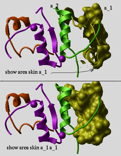
|
The area will be stored in r_out and the number of triangles used in the "skin" construction in i_out .
2.20.69.9 show atoms | [Top] |
shows properties of the selected atoms. Example:
build string "se ala" show surface area show a_//c* Atom Res Mol Obj X Y Z Occ B MMFF Code Xi Chrg formal Grad Area GrpThe fields:ca 1 ala a1 def -2.748 0.000 -2.245 1.00 20.0 1 113 C 1 0.06 0 0.0 0.5 _ a_def.a1/1/ca cb 1 ala a1 def -2.329 -1.202 -3.093 1.00 20.0 1 113 C 0 -0.09 0 0.0 7.3 _ a_def.a1/1/cb c 1 ala a1 def -4.247 -0.000 -1.935 1.00 20.0 3 121 C 0 0.45 0 0.0 34.2 c a_def.a1/1/c
| Field | Description |
|---|---|
| Atom atom name | |
| Res | residue number+[symbol] and name |
| Mol | molecule name |
| Obj | object name |
| X,Y,X | coordinates |
| Occ | occupancy (from 0. to 1.) |
| B | B-factor (positive) |
| MMFF | MMFF atom code |
| Code | ICM atom code |
| Xi | chirality number (0,1,2,3) |
| Chrg | partial charge |
| formal | formal charge |
| Area | solvent accessible surface area |
| Grp | electrostatic group (atoms can not be separated) |
| as_ | selection expression |
2.20.69.10 show atom type | [Top] |
shows atom types stored in the icm.cod file. The mmff option allows to check the Merck Force Field atom type.
Examples:
show atom type
# show all ICM types
-------------{atom codes}-----------
#
# icd vw hb hd wt sf na
#
atcd 0 0 0 0 0.000 0.00 ?
atcd 1 1 1 0 1.008 0.00 h
atcd 2 3 1 0 1.008 0.00 h
...
show atom type mmff "*cation*"
# cations
show atom type mmff "*iron*ion*"
# do we have iron ions?
show atom type mmff "?C=*"
# what types are connected to doubly-bonded carbon ?
show atom type mmff "[!C]*ring*"
# non-carbon types in rings
show atom type mmff 32
# some oxygens
-----------{MMFF atom codes}--------
Symb.Typ.[V] Description {formal charge}
O2CM 32 [1] oxygen in carboxylate anion
OXN 32 [1] N-oxide oxygen
O2N 32 [1] nitro oxygen
O2NO 32 [1] nitro-group oxygen in nitrate
...
2.20.69.11 show clash | [Top] |
shows all the interatomic distances between two atom selections which are shorter than the sum of van der Waals radii multiplied by the r_vwReductionRatio parameter (0.8 by default). IMPORTANT: this will work only for the ICM-objects. Use the show energy "vw" command (and pay attention to the current fixation) to precalculate interaction lists. The output will show the actual distance and the ratio of this distance and the sum of radii. Mark the two atoms of interest, separated by a logical OR, and paste it into another command if necessary.
See also: display clash, undisplay clash. Visualize the strained atoms with show a_//G or display a_//G .
Example:
build string "se ala his trp glu" randomize v_//* display show clash a_//c* a_//c* # clashes between carbons show clash a_//c* a_//c* 0.7 # more tolerant test display clash
2.20.69.12 show color list | [Top] |
shows list of colors defined in the file icm.clr and stores the output list in the S_out string array. Option mute suppresses output to the screen but still saves to the S_outarray (useful for scripts)
See also: color command.
An example:
show color
-------------{colors}-----------
1 black #000000
2 white #ffffff
3 grey #878787
4 blue #0065ff
5 red #ff0000
...
Example of show color mute use in a script:
if (Exist(view)) then # check if graphics is active
show color mute # saves a list of colors in S_out
for i = 1, Nof(S_out)
color background $S_out[i]
pause
endfor
endif
2.20.69.13 show arrays as parallel vertical columns | [Top] |
shows several arrays in a multi- column format.
See also: write column, show database, write database.
Example:
resnam = {"ala" "glu" "arg"}
reschg = { 0., -1., 1.}
show column resnam reschg
show column separator=":" comment="Example table" resnam reschg
2.20.69.14 show comp_matrix | [Top] |
shows residue comparison matrix used by the alignment algorithms.
See also: set comp_matrix, read comp_matrix.
2.20.69.15 show table in database format | [Top] |
shows several arrays or a table in a database format.
See also: read database show column, write database.
Example:
resnam = {"ala" "glu" "arg"}
reschg = { 0., -1., 1.}
show database resnam reschg
2.20.69.16 show drestraint | [Top] |
shows distance restraints. Arguments:
- optional as_select atom selection arguments specify atom pairs to be considered. Attention, the as_out selection can not be used as an argument since it is redefined by the command.
- r_violation : if the r_violation distance is specified, only the restraints deviating from the upper or lower bounds by r_violation are shown.
- center : If center option is specified the violation is measured with respect to the target value of the distance restraint and optionally only the distances greater than r_violation are reported.
- mute option: allows one to fill out the as_out selection and calculate the number of selected drestraints ( i_out ) without actually reporting them. It is useful for scripts.
Output:
- as_out atomic selection of all atoms for which the specified criteria have been satisfied
- i_out reports the number of selected drestraints
See also: drestraint and drestraint type.
2.20.69.17 show drestraint type | [Top] |
shows available drestraint types as defined in the icm.rst file. The numbered global or local types can be used to impose distance restraints. The other types are fixed and are used to impose disulfide bonds or peptide bonds.
2.20.69.18 show energy | [Top] |
calculates and shows values of currently set or explicitly defined in s_termString energy terms (e.g. "vw,el" ). If vs_ selection is specified, only the selected variables will be unfixed. The initial fixation will be restored after completion. Two additional atom selections may specify a subset of atom pairs that should be considered by the minimization procedure. Note that the contribution from the "14" energy term is not displayed separately. It is included in the "vw" contribution. If you want to display it separately, use the more straightforward Energy("14") function.
Important: the boundary element electrostatics is the most computationally heavy term. It is activated if electrostatic term el is switched on and preference electroMethod is set to "boundary element" . The most demanding part is the calculation of the boundary and its characteristics. Therefore, for multiple calculations with the same boundary we recommend to use make boundary and delete boundary commands.
2.20.69.19 show energy gradient | [Top] |
show gradient calculated by the minimize or show energy commands.
2.20.69.20 show hbond | [Top] |
calculates and outputs the list of hydrogen bonds. The real argument r_maxHbondDistance defines the upper bound of the distance between a hydrogen and a potential hydrogen acceptor to place the pair to the hydrogen bond list. Default value of r_maxHbondDistance parameter is 2.5 A. Number of identified hydrogen bonds is saved in i_out . To display/undisplay hydrogen bonds, use display hbond and undisplay hbond commands. Hydrogen bonds can also be calculated by the minimize and show energy commands provided that the hydrogen bond term is switched on.)
2.20.69.21 show bond exact | [Top] |
calculate the hydrogen bonding energy according to the distributed electron density geometry. Used in virtual screening to evaluate a score.
2.20.69.22 show table in html format | [Top] |
show the T_ table with HTML tags. Interpret web links according to the web link types described in the WEBLINK.DB array.
See also:
- write html s_file T_ [ link ... ] - write the html document to a file
- web T_ [ link ... ] - directly show the table in the web browser.
Example:
show html SR link SR.NA2 "PDB"
2.20.69.23 show iarray | [Top] |
show integer arrays defined in the shell. It shows names, dimensions and the first elements of arrays. The I_outarray contains the output of some functions and commands and is always in the shell.
ii={1 2 3 4 5 6 76}
iii=Count(10)
show iarray
---------------{iarrays}-------------
[1:1] { 0, ... }
ii[1:7] { 1, ... }
iii[1:7] { 1, ... }
2.20.69.24 show integers | [Top] |
show all integer shell variables. Example:
show integer
---------------{integers}------------
a 111
autoSavePeriod 10
defSymGroup 1
0
minTetherWindow 20
mnRemarks 3
mnSolutions 50
...
2.20.69.25 show label | [Top] |
show graphics string labels to find out their number. Then the labels can be addressed as label 1, label 2 etc.
See also: display string_label
2.20.69.26 show library | [Top] |
show loaded ICM-libraries. It's a lot of stuff, enter 'q' to exit.
2.20.69.27 show link | [Top] |
show links between sequences, alignments and corresponding molecules of 3D objects.
2.20.69.28 show logical | [Top] |
shows all logical shell variables in ICM-shell. Example:
aa=yes
show logical
---------------{logicals}------------
aa yes
yes
yes
no
yes
yes
...
2.20.69.29 show mol | [Top] |
shows selected atoms in the mol file format. See also: read mol and write mol.
2.20.69.30 show mol2 | [Top] |
shows selected atoms in the mol2 -file format (file extension .ml2). See also: read mol2 "file" and write mol2 "file" .
2.20.69.31 show molecule | [Top] |
shows all molecules of all objects currently in icm-shell. This command is identical to show a_*.*
2.20.69.32 show object | [Top] |
shows all molecular objects currently in icm-shell. This command is identical to show a_*.
The same result is achieved with the list a_*. command.
2.20.69.33 show pdb | [Top] |
show selected atoms in the PDB file format.
See also: read pdb "file", and write pdb "file".
2.20.69.34 show preferences | [Top] |
shows all icm preference variables in icm-shell (e.g. .
show preferences
..
atomSingleStyle = "tetrahedron"
1 = "tetrahedron" # current choice
2 = "cross"
3 = "dot"
..
2.20.69.35 show profile,rarray,real,sarray,string | [Top] |
shows all objects of specified type(s) in icm-shell. E.g. E.g.
show sarray rarray
2.20.69.36 show residue | [Top] |
shows all residues in all molecules of all molecular objects. This command is equivalent to
show a_*.*/*
2.20.69.37 show residue type | [Top] |
show names and characteristics of compounds described in the icm.res and user ICM residue libraries.
2.20.69.38 show segment | [Top] |
show segment representation of 3D structure of a protein for the selected molecules ms_ (all molecules of the current object by default).
See also assign sstructure segment, ribbonStyle, display ribbon.
2.20.69.39 show sequence | [Top] |
show all sequences or the specified sequence seq_ in one of specified formats. The default format is the fasta format. Option number defines if the residue numbers are added.
Three logicals: l_showSstructure, l_showSites, and l_showAccessibility control the display of a corresponding additional information aligned with the sequence.
Example:
read sequence "GTPA_HUMAN" show sequence swiss GTPA_HUMAN read pdb "1lbd" show surface area make sequence Info> sequence 1lbd_m extracted show 1lbd_m # you see relative accessibilities in 0-9 scale l_showAccessibility = no show 1lbd_m
2.20.69.40 show stack | [Top] |
show the following parameters of the conformations currently residing in the conformational stack.
- iconf - a slot number
- ener - total energy as calculated before the conformation was stored
- rmsd - the distance (either Cartesian or angular RMSD) between the current conformation of the object and the stack conformation calculated according to the compare command.
- naft - the number of visits AFTER the last improvement of energy
- nvis - the total number of visits to this slot; since new conformation are only compared with the last stack conformation the conformations may drift and cover a large area than described by the vicinity parameter
2.20.69.41 show table | [Top] |
shows the specified table in the ICM table format (one line per table row) or ICM database format (a list of column-name column values pairs for each entry). The header option suppresses the column subtitles.
See also: show html T_ . Database index tables are exceptions, show T_index will show all the entries of the related database. To see members of an index table type the index table name and press TAB.
2.20.69.42 show terms | [Top] |
shows the active energy/penalty terms. With option all it shows all the terms available. The result is saved in the s_out string. See also: set terms, delete terms.
2.20.69.43 show tethers | [Top] |
Shows tethered atoms with deviation larger than r_minDeviation (0. by default) and returns these atoms in as_out . Option mute is used when you just want to get a selection (as_out) of strongly deviated atoms.
See also: display tethers.
2.20.69.44 show version | [Top] |
show characteristics of the current ICM executable. Part of this string containing the version number is returned by the Version( ) function.
2.20.69.45 show vrestraints | [Top] |
shows vrestraints imposed on the internal variables of ICM molecular object.
2.20.69.46 show vrestraint type | [Top] |
shows types of vrestraints. These types are loaded from the icm.rst file.
2.20.69.47 show volume | [Top] |
Calculates the volume confined by the solvent-accessible surface or molecular surface (so called "skin"), respectively . Two optional selections [ as_1 [ as_2 ]] impose a mask on atom pairs, only those to be considered. If only the first selection is specified, the second one is assumed to be all atoms. The volume will be stored in r_out and the number of triangles used in the skin construction in i_out .
Examples:
read obj "small" show volume surface # inside accessible surface print "volume inside accessible surface = ", r_out show volume skin # inside molecular surface print "volume inside molecular surface = ", r_out
2.20.69.48 calculate volume of blobs of map density. | [Top] |
Contour electron density map at a given r_Threshold and calculate the volume of the high-density blobs. Defaults:
- take the current map;
- contour the whole map;
- use threshold value from the ICM-shell real variable mapSigmaLevel .
Examples:
read map "crn" # load m_crn map show volume m_crn 3. # calculate volume inside the
2.20.70 sort | [Top] |
[ sortarray | sortobjects | sortmolecules | sorttables ]
a family of sort commands (sort objects, molecules in ojbect, array/arrays or sort tables by their columns ).2.20.70.1 sort array(s) | [Top] |
sort one or several integer, real or string arrays. The first array is the sort key. By default ordering is lexicographic for string arrays and by increasing arithmetic value for integer and real arrays.
Options:
- reverse: reverse the sense of comparisons.
- number: enforce sorting according to arithmetic value for string arrays.
Examples:
a={3 2 1 5 7 4 6}
b=Sin(a*50.)
c={"three" "two" "one" "Five" "Seven" "four" "Six" }
show column a b c
sort a b c
show column a b c
sort reverse b a c
show column a b c
sort c b a
show column a b c
2.20.70.2 sort molecular objects by mass or a user field | [Top] |
resorts all molecular objects by the specified user field (see the set field command, and the Field function). If the field is not specified, the objects are sorted by their mass.
2.20.70.3 sort molecules in an object by mass or a user field | [Top] |
resorts the molecules in each of the selected non-ICM objects by the specified user field (see the set field command, and the Field function). If the field is not specified, the molecules are sorted by molecular mass. An ICM object can be stripped, resorted and then converted again.
2.20.70.4 sort table | [Top] |
[ sortstack ]
sort [ reverse ] [ number ] table.keyArray1 [ reverse ] table.keyarray1 [ reverse ] ...this command sorts all the arrays of the table so that all the listed table.keyArrays are applied sequentially with descending priority. Each array can be followed by the reverse option to change the sorting order.
Examples:
read table s_icmhome+"res.tab" # residue properties group table RES $s_out # create an ICM table RES sort RES.aa # resort entries by residue name show RES sort reverse RES.flexInd RES.aa show RES sort RES.hPhobInd RES.flexInd show RES
: sort stack
sort conformations in a stack according to their energies. New energies can be assigned to the same conformations with the set stack energy command.
2.20.71 split | [Top] |
[ splitgrob | splitobject ]
can split grobs or tables into individual components.2.20.71.1 split grob | [Top] |
[ splittable | splitcolumn ]
split g_complexGrob [ s_rootGrobsName] [ i_maxNofGrobs] [ r_minNofPointsInGrob ]divide disconnected parts of a graphics object into a bunch of separate graphics object sorted according to their size (measured as the number of vertices). The maximal number of new grobs is defined either by i_maxNofGrobs explicitly or by the MnGrobs parameter. The latter can be redefined in the icm.cfg configuration file. The i_maxNofGrobs option allows to retain only larger pieces. Grobs will be sorted according to their number of points and named by adding their sequential number to the input grob name or s_rootGrobsName, if specified.
The split command is used in protein cavity analysis and other applications where one needs to treat, display, and measure disconnected parts separately. You can also limit the number of points of the grobs generated by the command by providing the real argument with the minimal number of vertices you want in a grob.
See also: Volume( g_), Area( g_), Xyz( g_).
Example:
read object "crn"
make grob skin a_//cb a_//cb
split g_crn
display grob smooth # display as one smooth surface
undisplay g_crn
color grob unique
show Volume(g_crn3) Area(g_crn3) # you can also Ctrl-RightClick the grob
quit
# another session
read map "crn"
make grob
split g_crn "blob" 30 # create up to 30 largest grobs and
# call them "blob1" "blob2"...
# a variant: split g_crn "blob" 40 100.0 # discard grobs smaller than 100. vertices
delete g_crn
display grob
color grob unique
: split [ t_tableName]
split table into individual arrays.
Example:
group table t {1 2 3} "a" {2 3 4} "b" # t.a t.b arrays
split t # a and b arrays
: split [ tableColumn ] [ separator= character ]
takes each string of the specified column and splits it by the separator (comma is the default separator, e.g. separator="," ) The rows are multiplied accordingly. Example:
group table t {1,2} {"a,b,c","d,e"}
t
#>-A-----------B----------
1 a,b,c
2 d,e
split t.B separator=","
t
#>-A-----------B----------
1 a
2 d
1 b
1 c
2 e
Note that extra columns are appended to the original table (that explains somewhat
strange order).
2.20.71.2 Splitting an object into separate molecules | [Top] |
There is no such command, but if you want to split a molecular object into separate molecules, you can simply copy the object and delete unwanted molecules in each copy. Example:
copy a_ "b" delete a_b.!1 # delete all but the first molecule write a_b. "b" # contains only the first molecule # copy a_ "c" delete a_c.!2 # delete all but the second molecule write a_c. "c" # contains only the second molecule #etc..
2.20.72 sprintf | [Top] |
Print to the s_out string, or the s_outputStringName specified after the name= option. The same syntax as printf command, but the result is not displayed.
Example in which string outStr is the destination:
sprintf "mncalls = %d\n",mncalls name="outStr"
2.20.73 store | [Top] |
[ storeconf | storetorsion ]
store things to internal memory structures.2.20.73.1 store conf | [Top] |
store current conformation into specified slot of the conformational stack. By default it puts the conformation into the first free slot, or appends it to the end. The energy, by default, is automatically extracted from the previous energy evaluation, or taken from r_energy if explicitly provided. The total number of visits ( nvi ) is set to 1 by default, or Example:
buildpep "WSD" montecarlo # generates a stack show stack set v_//omg 180. # change a conformation store conf -9. # add conformation with energy -9. store conf 3, -9. # override slot 3 with energy -99. store conf number=33 # set conf with number of visits=33
2.20.73.2 store conf | [Top] |
store temporary torsion types for new ICMFF potential for a given molecule (not used in the commercial distribution).
2.20.74 ssearch | [Top] |
- you may globally optimize any set of energy/penalty terms including electrostatics, solvation, entropy, density correlation etc.
- you may search an arbitrary subset of variables
- you may allow full local minimization after each systematic change
- you may search only through centers of the preferred local multidimensional zones (for example rotamers) which is more efficient than an even grid sampling
- you may perform both the global search (the full [-180.,180.] range) and the local search ( grid search around the current conformation).
ssearch [ local ] [ vs_Ssearch [ vs_minimize ]] [ as_select1 [ as_select2 ]]
systematically changes vs_Ssearch variables and carries out energy minimization with respect to the vs_minimize variables after each systematic conformational change. The lowest energy conformation is loaded from the conformational stack at the end of the procedure. By default every variable from vs_Ssearch selection goes through nSsearchStep evenly distributed values. The step therefore is 360 deg. over nSsearchStep. Option local imposes the grid locally around the current values of vs_Ssearch variables. In this case the program uses ssearchStep parameter.
If you want to prevent the procedure from automatically writing the stack of best conformations to a file set the autoSavePeriod variable to zero.
See also montecarlo .
Example:
read object "crn" # good old crambin ssearch v_/14/x* # place optimally Asn14 side-chain
2.20.75 strip | [Top] |
strip an ICM-molecular object from its ICM attributes and reduce it into a pdb-object. The latter are still good for graphics, superposition, basic geometric manipulations etc. Also, some chemical operations, e.g. attaching chemical groups are best performed on simpler pdb-objects. Stripping may save you a lot of memory as well.
Option virtual tells the command to delete the virtual atoms upon convertion. The virtual atoms ( selected as a_//vt* ) are always present in the ICM object, but are not necessary in the stripped object.
String is also used to perform operations which are not allowed for ICM object, but are allowed for simpler PDB objects (for example dragging individual atoms with a mouse)
These commands include:
- deleting hydrogens
- make bond auto
Example:
build smiles "c1ccccc1" strip a_ virtual
2.20.76 superimpose | [Top] |
[ alignmentoptions ]
superimpose [ [ align | ali_ ] [ exact ] ] as_selectStatic as_selectMovablesuperimpose os_static I_atomNumbers1 os_movable I_atomNumbers2
superimpose as_movableByTethers
optimally superimpose the second movable object onto the first one using selected atoms or residues as equivalent points. At least one pair of equivalent atoms needs to be provided.
Selections may by of any level: atom selection as_ residue selection rs_ molecular selection ms_ or object selection os_ . The option defines how the two sets are aligned (the residue alignment may be explicitly provided as the ali_ argument, and the objects are linked with the alignment):
alignment options:
- Default (no options): Residue alignment: by residue number. Atom alignment: by atom name for pairs of identical residues or pairs of close residues (F with Y; B with D,N; D with N; E with Qor Z, Q with Z), for other residue pairs only the backbone atoms ca,c,n,o,hn,ha are aligned.
- align option: Residue correspondence is established by sequence alignment using the ICM ZEGA alignment Abagyan, Batalov, 1997 Atom alignment: by atom name (see the default option).
- exact option: Residue matching is ignored. Two atom selections are directly sequentially aligned. Numbers of atoms in two selections must coincide.
- align exact option: Residue alignment: Needleman and Wunsch. Inside residue atoms are aligned sequentially and regardless of the name.
Number of equivalent atom pairs is saved in i_out; resulting RMSD is saved in r_out; a selection of atoms in the "static" object used for superposition is saved in as_out, that of "movable" object in as2_out .
Virtual atoms. Be default, the first two virtual atoms ( vt1 and vt2 ) are automatically excluded from both selections unless the virtual option is explicitly specified.
Note that if the movable object is of ICM-type it is preferable to have all six virtual variables unfixed ( e.g. unfix V_movableObj.//?vt* ). Otherwise, if some or all of them ( V_//?vt* ) are fixed, you will get a warning, and only the partial minimization of the RMS distance possible with the given degrees of freedom will be performed.
If the explicit order of atoms is specified and two single object selections are provided, e.g.
superimpose a_a. a_b. {3 5 7} {10 3 5}
the superposition will be performed in the specified order.
See also: Rmsd( ), Srmsd( ).
2.20.77 sys (or unix): system command | [Top] |
issues a system shell command from ICM. You may use sys or unix interchangeably. By default, the ICM process waits until the system shell process has completed. sys must be the first word in the command. Important: Construction
if ( <condition> ) sys system_commandis illegal. Use
if ( <condition> ) then
sys system_command
endif
instead.
For cross-platform compatibility, also use the following portable
ICM shell variables instead of non-portable system-specific commands:
s_sysCp, s_sysLs , s_sysLtt, s_sysMv, s_sysRm
Example:
sys $s_sysCp # cross-platform portable list command sys ls # non-portable unix only ls command
As you might have guessed from the above example, to pass the ICM-shell variables to the system_shell_command one may use integer, real or string ICM-shell variables, protected with dollar sign ($) prefix. Important: passing ICM-shell variables to the UNIX command is impossible if you use an alias name (e.g. ux) instead of the original unix command.
Examples:
unix grep -i myoglobin /data/pdb/brookdir.doc
unix echo $mncalls $s_pdbDir $dielConst
file="/data/pdb/"+Name(a_1.) # tricky file name
unix grep ATOM $file | wc -l # $file will be substituted by
# the value of this ICM-shell
# string variable
2.20.78 then | [Top] |
See also if, elseif, and endif .
2.20.79 transform | [Top] |
transform {ms_|g_grob} R_12transformationVector
transform molecules ( ms_ ) or graphics objects according to the transformation vector.
See also these two examples: ( example 1 and example 2).
You can also manually move molecules with respect to each other on the graphics screen by using the connect ms_ command to choose the molecules which can be moved separately.
transform [copy] ms_ [i_number] [s_symgroup] {box|as_selection r_radius}
transform molecules ms_ according to the specified transformation. i_number is a symmetry operation number in an array of all operators of a space group. The symmetry transformations are defined in a 12*n real array where each chunk of 12 real values defines 3x3 rotation matrix and translation vector {a4,a8,a12}. The complete 4x4 transformation matrix looks like this:
a1 a2 a3 | a4 a5 a6 a7 | a8 a9 a10 a11 | a12 ------------+---- 0. 0. 0. | 1.If i_number exceeds the number of space group symmetry transformations the symmetrical images in up to 26 surrounding cells are created. This operation is only possible, if symmetry information (sym.group name and cell dimensions) is defined for the object. Usually PDB and CSD files contain the above information, it is preserved upon conversion. Use the Cell( ) or the Symgroup( ) functions to find out if the space group is defined. If not, you may assign it to the object with the set symmetry object command. In a special case of i_number=0, the object is placed in the "primary" subunit of the cell (e.g. in sym.group "P 21 21 21" that is 0<x<a, 0<y<b, 0<z<c/4; currently, the i_number=0 option is supported only for groups 1 and 19).
Example:
read mol2 "ex_mol2" # several small molecules display a_4. build hydrogen a_4. # added and displayed
2.20.80 translate | [Top] |
translate the center of mass of the specified object(s) ( os_ ) or molecule(s) ( ms_ ) to a specified position, or by a R_3translationVector vector if option add is specified. You can also move molecules/objects interactively with the mouse after the connect command.
symmetry option With the symmetry option the R_3translationVector should be in fractional coordinates. Option add translates by the specified vector from the current position. Without add the program tries to identify a compensating shift to a position in which the center of gravity of the selected molecule(s) has minimal positive fractional coordinates.
Examples:
read pdb "1fbi"
delete a_!p,q,y # get rid of reduncancies
cool a_
for i=1,10
translate a_y i*{0., 0., -0.5} # shift molecule y by an increment
endfor
To calculate a displacement vector, following this example in which we calculate a translation vector for molecule y :
read pdb "1fbi" delete a_!p,q,y # get rid of reduncancies cool a_ v1 = Rarray( Xyz( a_y/1/ca ) ) connect a_y # no drag the molecule with the middle button and press Esc v2 = Rarray( Xyz( a_y/1/ca ) ) v_trans = v2 - v1
2.20.81 undisplay | [Top] |
undisplay window
Examples of the undisplay command:
undisplay ribbon # ribbon display not needed any more undisplay g_icos # a graphics object not needed any more undisplay a_/w*,hoh* # who cares about water molecules ... undisplay residue labels # just "labels" will do the same undisplay string # see also "delete label" command undisplay a_//h* # who cares about hydrogens ... undisplay hbond a_1./1:29 # ... and, hence, about H-bonds undisplay tether a_/12:20 undisplay box undisplay cursor undisplay origin # undisplay the coordinate frame undisplay window # delete GL graphics window
2.20.82 unfix | [Top] |
unfix (set free) specified variables (such as bond lengths, angles and phases or torsions) in an ICM-object. Opposite to fix command. This operation can be applied to the current object only (use set object os_newObj first).
Important: since it only makes sense to unfix variables which are currently fixed, use Vs_selectwhich selects among ALL (both free and fixed) variables, as opposed to vs_ which selects only from FREE variables.
Examples:
# only this loop has free torsions now
unfix only V_/8:18/phi,PSI,H,M,P
Note that PSI torsion references is used for traditional residue attribution
2.20.83 wait | [Top] |
wait
allows to synchronize multiple ICM processes spawned by the fork command.
- for the parent process: wait until all the child processes spawned with the fork command are finished.
- for the child processes: quit the spawned ICM process
2.20.84 web | [Top] |
a family of web commands.
web [ delete ] u_EntrezRequest
invoke a web browser call to the WWW page of the Entrez server at NCBI and display your database entries with links. The format of the requests is described at http://www3.ncbi.nlm.nih.gov/Entrez/linking.html. The s_webEntrezLink string defines the location of the link and the webEntrezOption preference defines the type of the Entrez report. The delete option will temporarily set l_confirm=no for this command.
Examples:
web sp||GTPA_HUMAN # Swissprot by ID web sp|P07497| # Swissprot by accession web emb|U01234| # EMBL by accession web pdb|1crn| # PDB by ID (a single chain entry) web pdb|2ins|a # PDB by ID and chain character web 1111111 # NCBI nonredundant database
2.20.85 web table: shows an icm table with a web browser | [Top] |
ICM invokes a web browser call. If you do not have a browser (defined by the s_webViewer string) currently running under your login, the call will fail. The command presents the T_ table in your web browser window. Optional web links are interpreted according to the web link types described in the WEBLINK.DB array.
If the table contains chemicals, ICM creates a file with the compound images using Peter Ertl's JME classes (see also the s_javaCodeBase variable).
See also:
-
`writehtml{write html [s_file] T_ [ link ... ]}- write the html document to a file -
`showhtml{show html T_ [ link ... ] }- show the table in the icm text window.
Example:
show html SR link SR.NA2 "PDB" # read sequence "GTPA_HUMAN.seq" find profile show SITES web SITES web SITES link SITES.AC "AUTO"
2.20.86 while | [Top] |
is one of the ICM flow control statements, used to perform a loop in the ICM-shell calculations.
See also: for, endwhile .
2.20.87 write | [Top] |
[ writealignment | writebinary | writeiarray | writearray | writedrestraint | writedrestrainttype | writefactor | writegrob | writehtml | writeimage | writeindex | writeindexblast | writelibrary | writemap | writemodel | writemol | writemol2 | writeobject | writeobjectsimple | writepdb | writepostscript | writepov | writesegment | writesequence | writesession | writestack | writevs_var ]
write stuff to a disk file. Logical variable l_confirm defines if you'll be prompted whether to overwrite an existing file with the same name. Use option delete to delete (or overwrite) the existing file unconditionally.For the list of ICM-objects you can write, and formats you can choose, see read and show commands. Generic syntax:
write [binary] [ append | delete ] { variable | constant | expression } s_fileNameRoot[.ext]
With the binary binary option multiple objects or classes of objects can be writtin into a single cross-platform compatible binary file.
See also corresponding read commands.
2.20.87.1 write alignment | [Top] |
write alignment ali_Name to a file. Default extension is .ali . Note: if alignment is only a group of unaligned sequences, generated by the group command, the result will be just a multiple sequence file, rather than an alignment file (there will be no dashes at the end).
The default ICM format for an alignment looks like this:
#>ali sh3 # Consensus ...#.^.YD%..+~..-#~# K~-.#~##.~~..~WW.#. ~~.~ Fyn ----VTLFVALYDYEARTEDDLSFHKGEKFQILNSSEGDWWEARSLTTGET Spec DETGKELVLALYDYQEKSPREVTMKKGDILTLLNSTNKDWWKVE--VNDRQ Eps8 KTQPKKYAKSKYDFVARNSSELSM-KDDVLELILDDRRQWWKVR---NSGD #Fyn __EEEE__________________EEEEEEE____EEEEEE_____E # Consensus G%#P...#..#. Fyn GYIPSNYVAPVDSIQ Spec GFVPAAYVKKLD--- Eps8 GFVPNNILDIMRTPE #Fyn EEEGGGGEEE_____ # nID 7 Lmin 61 ID 11.5 %
The lines starting from hash (#) are comments and are not required
The length of each alignment block is controlled by the sequenceLine parameter (default value is 60). If you want to save a long alignment as one unwrapped block, increase this value (e.g. sequenceLine=1000 )
Writing sequences in the alignment order
The sequences can be written in the alignment order with the following commands (they can be store in a little macro)
macro wrSeqAli ali_ s_file ("seq.fasta")
l_showSstructure = no
seqname = Name(ali_) # Name returns sarray of sequence names
for i=1,Nof(seqname)
write sequence fasta append $seqname[i] s_file
endfor
endmacro
Resorting alignment in the order of sequence input.
Upon alignment the source sequences get reordered according to similarity. If you want to keep the original order you may use the reorderAlignmentSeqmacro described in the Align ali_ I_newOrder ) section and then write an alignment:
read sequence s_icmhome+"zincFing" group sequence aaa align aaa reorderAlignmentSeq aaa write ali_new # reordered alignment
See also: String( ali_) function.
2.20.87.2 write binary | [Top] |
write specified ICM shell objects or all objects of a classes to a single, binary, cross-platform file, or more accurately, database. The following data types are currently supported:
The catalogue of the database can be obtained with the list binary command. The default file name is "icm.icb", and the default extension is .icb (stands for ICm Binary file). The system objects or the objects with property
Examples:
-
ii = {2 3 4}
rr = {2. 3.4 5.5}
g = Grob("CELL",{1. 1. 1.})
g2 = g*2. # twice as large
write binary iarray rarray grob # the default file is icm.icb
Info 4 icm shell objects icm.icb
list binary # looks at "icm.icb"
1 ii iarray 20
2 rr rarray 32
3 g grob 1788
4 g2 grob 1788
delete ii
read binary name={"ii"}
Info 1 icm shell objects read from icm.icb
write binary grob "aaa"
Info 2 icm shell objects aaa.icb
See also: list binary, read binary
2.20.87.3 write iarray | [Top] |
[ writerarray | writesarray | writematrix ]
write [ iarray ] I_name [ s_fileName ]!_ write rarray
write [ rarray] R_name [ s_fileName ]
!_ write sarray write [ sarray] S_name [ s_fileName ]
!_ write matrix write [ matrix ] M_name [ s_fileName ]
write an array or a matrix to a disk file. Default file extensions are .iar, .rar, .sar, or .mat, respectively.
See also: read iarray, read rarray, read sarray, read matrix.
2.20.87.4 write several arrays | [Top] |
[ writetether | writetable | writetablemol | writecolumn | writedatabase ]
write [ { column | database ] } array1 array2 .... [ s_fileName ]write arrays in the column or database format to a disk file. Default file extension is .db
See also: read database.
!_ writing tethers
If you imposed tethers between you current object and another object and you want to quit the session and then restore you setup, you can use the following trick:
-
# first let us create an object a_ly6. tethered to template a_x.
read alignment s_icmhome+"sx"
read pdb s_icmhome+"x"
build model ly6 a_x.m # a new object a_ly6. created and tethered
#
write string String( a_//T ) "tTz.str" # tethered model atoms
write string String( a_//Z ) "xTz.str" # x-template atoms
write object a_x,ly6. "tx.ob"
#
quit
#
% icm
read object "tx.ob"
read string "tTz.str" name="tTz"
read string "xTz.str" name="xTz"
set tether $xTz $tTz exact # tethers restored
!_ write table
writing ICM table in text format write T_table1 [ T_table2 .. ] [ field= s_delimiter ] [ s_fileName ]
write the T_table table to a disk file *.tab. It will have two header lines with table name and field name information, followed by the values.
The default extension .tab is appended automatically. The ICM text table format has a header which allows to read this table back to icm with the read table command
Example:
group table t {1 2 3} "a" {"one","two","three"} "b"
t1=t[2:3]
write t t1 "tt" # write both tables in one file
delete table # read both tables
writing tables in CSV or TSV formats
write T_table1 [ header ] [ separator= s_delimiter ] [ s_fileName ]
if the separator or the s_fieldDelimiter variable contain just a simple symbol (e.g. comma or tab), ICM will write a comma-separated or tab-separated table with the first line containing the field names, e.g.
group table t {1 2 3} "a" {"one","two","three"} "b"
write t header separator="," "t.csv"
unix cat t.csv
a,b
1,one
2,two
3,three
write t separator="," "t.csv" # without header
unix cat t.csv
1,one
2,two
3,three
To read a table in comma-separated format with the headers, use the following commands:
read table separator="," header name="t" "t.csv"
writing tables in a binary format
write binary T_table1 T_table2 .. s_file write binary tables s_file
The most compact and fast format is the binary format. Any object can be saved to and read from a binary project file with ".icb" (ICM-binary) extension.
See also write database T and write column.
: write table mol
writes an ICM chemical spreadsheet as a mol/sdf file. All the property columns are added as feature records to individual mol-entries. Option index adds sequential order number as an additional property named IX (it may be useful as an ID).
Example:
read table mol "ex_mol.mol" name="t" unique write table mol t
!_ write column
write column array1 array2 .... [ s_fileName ] [ separator= s_Separators]
write arrays in a multi- column format to a disk file.
Examples:
read column s_icmhome + "res.tab" # amino acid properties write column aa flexInd "tm.tab" # two columnsIf you want to write all the entries of an ICM-table you may do the following.
Examples:
read column s_icmhome + "res.tab" # a set of isolated arrays group table RES $s_out # create an ICM-table RES (s_out : array names) write RES # write in the 'table' layout write database RES # write table RES in the 'database' layoutDefault file extension is .col.
See also: read column, show column. read table, show table.
!_ write database
write database [ html ] { array1 array2 .... | table } [ s_fileNameRoot ]
write several arrays or a table in a database format to a file (usually tables are written in a multi column format). This command can also be used to save a subset of arrays of a table in a specific order. Option html writes the table with appropriate HTML tags. See also read database write table, show database.
Example:
resnam = {"ala" "glu" "arg"}
reschg = { 0., -1., 1.}
write database resnam reschg "a" # default extension ".db" will be added
#
group table t resnam reschg
write database t.reschg t.resnam "a" # reverse the order</tt>
2.20.87.5 write drestraint | [Top] |
write distance restraints of the current object to a file.
See also: drestraints and drestraint types.
2.20.87.6 write drestraint type | [Top] |
write drestraint types to a file. You may define your own types with the set drestraint type command or by editing a *.cnt file.
2.20.87.7 write factor | [Top] |
writes crystallographic structure factors to a file.
2.20.87.8 write grob | [Top] |
write/append a graphics object (grob) to a disk file. If g_name is not specified, all grobs are written. Default file extension is .obj
See also: write image, write postscript.
2.20.87.9 write html | [Top] |
writes the T_ table with HTML tags to a file. Interpret web links according to the web link types described in the WEBLINK.DB array. If the table contains chemicals, ICM creates a file with the compound images using Peter Ertl's JME classes (see also the s_javaCodeBase variable).
See also:
- show html T_ [ link ... ] - show the html formatted table in the text window
- web T_ [ link ... ] - directly show the table in the web browser.
- s_javaCodeBase - path to Java applet classes.
Example:
write html SR "results.htm" link SR.NA2 "SP" # link to Swissprot
2.20.87.10 write image | [Top] |
write the current screen image to a file. The default image file format is tif . The png-format is the most compact and is recommended for web-publishing. The default settings are stored in the IMAGE table. Some of them can be overridden by the following options:
- display - allows to view the saved image or postscript image file. The viewer is defined by the s_imageViewer variable for targa, gif, rgb and tif images and by the s_psViewer variable for the postscript images.
- postscript - write Adobe postscript-bitmap file rather than TIFF-file. See also write postscript command which generates vectorized scalable high quality postscript files.
- preview - add low-resolution preview to postscript file for some EPS-compliant image viewers (i.e. Irix showcase®). Resolution, and therefore the size, of the added preview is defined by the IMAGE.previewResolution (default 10).
- print - print the postscript file. It will not work for non-postscript images, in which case you may use the display option and print from your image viewing program instead.
- compress - use packbits lossless compression standard for .tif files. Compression of this kind is currently a standard feature of all baseline TIFF-reading programs. Compression is a standard feature of the .gif and .png formats.
- stereo - generate stereo image even from the mono display. Tiff-files preserve the image screen dimensions for each image in a stereo-pair. Stereo-base for postscript files is controlled by the IMAGE.stereoBase parameter and equals 2.35" (60mm) by default.
- color or bw - color or black-and-white options surpass IMAGE.color logical variable.
- window= I_xyPixelSizes - generate image of any
arbitrarily large resolution (e.g. window=3*View(window) to triple the resolution).
Suppose that you want to make a poster
of 4613 by 2888 pixels. This resolution is not achievable on a 1200x1024
screen. The image area will be divided into many squares and the program
will merge them into one image of large resolution. This option will
not work with string labels.
Example:
nice "1crn" # resize the image delete label IMAGE.compress = no #just a plain uncompressed image write image window={4000,2700} # for slides write image window=2*View(window) # double the res.
IMAGE.generateAlpha logical variable controls if the alpha channel information is added to the SGI rgb and tif image files. This additional channel describes opacity of the image pixels and makes the background transparent. Images generated with alpha channel can be nicely superimposed in the IRIX showcase since their backgrounds are transparent.
Examples:
display a__1crn. ribbon write image "a" # a.tif image - about 1400 kB write image "p" compress # p.tif image - about 88 kB write image postscript stereo display "aaa.eps" write image 2*View(window) # hi-res, may screw up labels unix lp -c a.eps # print if you like the resultSee also: write grob, write image , write postscript.
2.20.87.11 write index | [Top] |
calculate and write index for a database file described by the control table T_dbDescription. This table, optional for mol/sdf files, contains information about the database file (files) and fields to be indexed. It may have the following components in the header:
- DIR - string directory name
- FI - sarray of database files
- EXT - extension of the database files
Example:
group table t {"ID","DE","KW","SQ"} "fd" header "/data/swissprot/" \
"DIR" {"sprot"} "FI" ".dat" "EXT"
# we created control table t
write index swiss t "/data/icm/inx/SWISS.inx" # make index and save to a file
read index "/data/icm/inx/SWISS.inx" # read index
show SWISS[2:5]
show SWISS.ID=={"12AH_CLOS4","1431_LYCES","B3AT_CHICK"}
read sequence SWISS.DE=="DNA-BINDING"
2.20.87.12 write index blast | [Top] |
create a set of blast-formatted binary files for searches with the find database command. The command will use all the sequences currently loaded into the ICM-shell and will create the following compact binary files (the first three files are the same as those generated by the setdb blast command):
- name.bsq binary sequences
- name.atb pointers
- name.ahd sequence headers
- name.bsa relative solvent accessibilities for each residue. This information
find database write s_DBpath output= s_fastaFile
command.
Simple example (indexing can also be done with the blast setdb routine):
read sequence "aaa.seq" # fasta formatted
write index sequence "./aaa"
delete sequences
a=Sequence("SFDGHASGDFSHGASFDHAGS")
find database a "./dom" 0.001
An example in which the sequences+accessibilities are generated from objects:
read sarray "domain.list" name="dom" # e.g. {"1crn","1abc.a/12:115/",..}
for i=1,Nof(dom)
read object s_icmhome+"data/xpdb/"+dom[i]
show area surface mute # calculate the absolute acc. areas
make sequence a_1 # the relative areas are calculated and assigned to seq.
delete a_*.
endfor
write index sequence "./dom" # files .bsq .atb .ahd .bsa created
delete sequences
2.20.87.13 write library | [Top] |
save a selected molecule, residue or a fragment as an ICM-library entry. Use set charge, set bond type and, possibly, build hydrogens before writing an entry. We recommend you to do this operation in an interactive session: display your molecule and Ctrl-Click the first and last atoms if needed. There are two different situations:
- the molecule/residue/fragment does not belong to an ICM-type object. For example, you have a pdb-file with a new molecule you would like to create an ICM-library entry from. In this case do NOT use option auto and note that the resulting entry will only be a draft, since energy parameters of atoms ( atom codes plus related types of van der Waals, hydrogen bondings solvation ), as well as parameters of torsions, bond angles, phase angles, and bond lengths will have to be further manually adjusted. Enter the command and you will be prompted for the first and the last atoms of the entry. The purpose of this procedure is to create a regular ICM-tree, create extra bonds if there are cycles and give atoms unique names. Some additional editing of the entry may be required to correct fixed and free torsions suggested by the program. To declare a certain variable free, enter '+' in the appropriate field.
- the molecule/residue/fragment belongs to an ICM-type object. In this case you may use option auto since all the information is there already. The program only needs to extract the molecular subtree according to the specified selection.
Example:
BS nter glu cooh # build glutamic acid residue strip # convert it to a non-ICM object write library a_def.a1/1/hg2 "./tm" name ="new" auto # reroot it # Now the entry atom is a_//hg2 build string "se new" library ="./tm" # read the rerooted residue display
2.20.87.14 write map | [Top] |
write specified map to a binary file with specfied file.
write { map | m_map1 m_map2 ... }
write all maps or specified maps to corresponding files ( the names for the files are generated from map names, the m_ prefix is removed from the file names).
write xplor m_map ... [ s_fileName ]
write the specified map to a Xplor-formatted file.
Example:
make map "ge,gc" potential Box(a_) m_gc... done Info> Map m_gc created. GridStep=0.50 Dimensions: 16 11 17, Size=2992 m_ge... done Info> Map m_ge created. GridStep=0.50 Dimensions: 16 11 17, Size=2992 write m_ge m_gc Info> 1 map written to file ge.map Info> 1 map written to file gc.map
2.20.87.15 write model: update or create the loop database file | [Top] |
writes a compressed representation of the protein structure to the specified loop file ( "def.lps" by default ). To create a large database, read the object list and write a loop over all objects, e.g.
# prepare pdbUniq list and .. read sarray "pdbUniq.li" for i=1,Nof(pdbUniq) read object s_xpdbDir+pdbUniq[i] # add further filters write model append "icm.lps" delete object endfor
To make the program use this file , redefine the LIBRARY.lpsfile name to, say "./icm.lps"
2.20.87.16 write mol | [Top] |
write selected atoms in the mol -file format. By default the formal charges (see the set charge command) are saved. Options
- exact: preserve the ICM-atom names (like c1, c2).
- charge: write the MCHG section containing the atomic real charges.
See also read mol "file", show mol "file".
2.20.87.17 write mol2 | [Top] |
write selected atoms in the mol2-fileformat (extension .ml2). Options:
- exact preserves the ICM-atom names (like c1, c2).
- formal writes formal atomic charges instead of the real ones. Adds USER_CHARGES (XXXXXX) tag to the header
See also read mol2 "file", show mol2 "file".
2.20.87.18 write object | [Top] |
write an ICM molecular object (or many selected ICM-objects) in binary ICM format to a file. A single object can be renamed in the file according to the s_fileName, if option rename is specified. Important: only whole ICM object may be written by this command, and file extension will always be .ob.
Options (defaults shown in bold):
- append : append to a multiple-object file
- rename : rename the single object to s_fileName (leave out path and extension) .
- short : write a compressed file for non-ICM objects without b-bactors and occupancies.
- strip : write a stripped object (i.e. drop information about variables and rigid bodies present in an object of the ICM type).
- auto={yes| no} : if yes the program automatically identifies which atom requisites to save. For example, if molecule is displayed, the view will be saved with the object. Properties such as occupancy and charge are considered essential if the values are not identical for all the atoms. If auto=no, the OBJECT table controls the output.
- occupancy={yes|no} : occupancy field
- charge ={ yes|no} : partial atomic charges
- bfactor ={ yes|no} : b-factors
- display ={yes| no} : the current view of your molecular object(s), including graphics planes The written display attributes are automatically restored upon reading of the object.
- library={yes|no} : currently not used.
Example:
read object "crn" build string "se ala his" name="AH" # second object named "AH" write object a_2. "alahis" rename # rename obj. to "alahis" display a_1./1:40 ribbon # display and save with graphics attributes display a_1./12 cpk display a_2. xstick write object a_*. "twoobj" display=yes # both objects in one file write object a_1. append "twoobj" # yet another object
2.20.87.19 write object simple | [Top] |
write a compressed object. The information preserved in the compressed description of the object is limited to 3 coordinates and certain atom names (non-protein atom names will not be preserved and reduced to just one character) plus all residue and molecule requisites. For a PDB-type file, a simple object is the most compact for store and fastest to read. They are used in the compact fold library.
2.20.87.20 write pdb | [Top] |
write a molecular (sub)object in PDB format. Normally atoms of each amino acid are sorted in the following order:
ATOM 19 N GLN O 3 -4.565 0.000 -4.592 1.00 20.00 ATOM 20 CA GLN O 3 -4.712 0.000 -6.037 1.00 20.00 ATOM 21 C GLN O 3 -6.194 0.000 -6.420 1.00 20.00 ATOM 22 O GLN O 3 -7.063 0.000 -5.549 1.00 20.00 <i>the rest</i>Also the n-terminal nitrogen and its hydrogens are assigned to the first amino acid. Options are the following:
- charge saves atomic charges instead of occupancies and atomic radii instead of B-factors;
- exact keeps the names of hydrogen atoms the same
as in ICM objects (i.e. the first character is 'h'). Without this option
names of hydrogen atoms are transformed like this:
h11 ==> 1H1 h12 ==> 2H1
- nosort retain the original ICM order of atoms
See also: write object, read pdb.
2.20.87.21 write postscript | [Top] |
create vectorized postscript model of the screen image. Instead of the bitmap snapshot this command generates lines, solid triangles and text strings corresponding to the displayed objects. Since the postscript language is directly interpreted by high-end printers, the printed image may be even higher quality than the displayed image. The final resolution is limited only by the printer since the original image is not pixelized. Warning: there may be inevitable side-effects for some types of solid images at the intersection lines of solid surfaces (i.e. large scale cpk-representation hint: use display skin instead).
The default settings are stored in the IMAGE table. Some of them can be overridden by the following options and arguments:
- reverse - makes white background in the saved postscript file.
- display - allows to view the saved postscript file. The viewer is defined by the s_psViewer variable.
- stereo - generate stereo image even from the mono display. Stereo-base is controlled by the IMAGE.stereoBase parameter and is 2.35" (6cm) by default.
- preview - generates postscript preview according to the IMAGE.previewer command string and the IMAGE.previewResolution parameter.
- color or bw - color or black-and-white options surpass IMAGE.color logical variable.
- dash - is a great variant of the black-and-white option to generate lines of
different width and style. The line colors of your screen image are interpreted according to the
following table:
- gold - double solid black line
- pink - triple solid black line
- magenta - dash1
- orange - dash2
- brown - dotted line
- the rest - solid black line
display a__crn. # display wire model of crambin color a_//ca,c,n pink # triple width backbone color a_/arg/!ca,c,n magenta # dashed lys side chains # zoom your picture to fill the whole graphics window write postscript dash stereo display
- i_quality (default=3, possible range: 1:100) - defines a parameter in a smoothing procedure. Each side of an elementary triangle is divided into i_quality sections and color of all the i_quality2 smaller triangles is calculated to yield smooth transitions. Optimal value of the parameter depends on an image. Only large scale images may require i_quality values above 10. Only in an extreme case of a single triangle on a page with red, blue and green vertexes, one may need i_quality of 100.
- r_gammaCorrection allows to lighten or darken the image by changing the gamma parameter. A gamma value that is greater than 1.0 will lighten printed picture, while a gamma value that is less that 1.0 will darken it. You may adjust your gamma correction parameter for your printer with respect to your display and add this setting to the _startup file.
Examples:
display a__crn. brown skin # molecular surface
# Hugh wants to have a look
write postscript 1 1. "divine_brown" display
# change parameters for the printer
write postscript 5 2. "divine_brown"
# and print it
unix lp -c divine_brown.eps
See also:
write image,
write grob.
2.20.87.22 write pov | [Top] |
writes a pov-ray object file which can be processed with the pov-ray ray-tracing program.
Example:
buildpdp "ala his trp" display cpk make grob image write pov "x" % pov-ray x.pov
2.20.87.23 write segment | [Top] |
writes a simplified description of protein topology generated by the assign sstructure segment command to a file. You can append your description to the provided foldbank.seg file.
Examples:
read object "crn" assign sstructure segment a_* write append segment "myseg"See also: find segment, read segment.
2.20.87.24 write sequence | [Top] |
write all sequences or the specified sequence seq_ to a file in one of specified formats. The default format is the fasta format.
2.20.87.25 write session | [Top] |
write commands from an ICM session to a file. Default file name is "_session.icm". This is a simple text file with icm commands. Feel free to edit the file
Example:
.. a=1 history 10 write session Info> 4 history lines written to file _session.icm
See also: history and delete session commands.
2.20.87.26 write stack | [Top] |
write the current state of the conformational stack to a disk file. Starting from May, 2003, version ICM3.022, the stack file is compressed by default. The stack file is not compressed if the simple option is used. Default file extension is .cnf.
See also: show stack, delete stack, read stack, read conf.
2.20.87.27 write vs_var | [Top] |
write a variable selection vs_ to a disk file.
Default file extension is .var .
See also: read variable.
| Prev vs_out | Home Up | Next icmfunctions |