| Contents |
|---|
| Introduction |
| Reference Guide |
| User's guide |
| References |
| Glossary |
| A |
| B |
| C |
| D |
| E-H |
| S |
| T |
| U-Z |
| Index |
| Prev | 5.6 S | Next |
[ site | grob | hbond | svariable | integer | label | logical | macro2 | map | matrix | mimel | mmff | mol | mol2 | more | movie | mute | only | parray | pattern | png | patternmatching | pdb | peptide | profile | prosite | rebel | real | regularization | residue | rgb | ribbon | script | sequence | segment | shell | skin | smiles | sln | stack | stick | string | factor | surfacearea ]
!- site ICM sequences and objects may contain specific information about local sequence features, such as location of binding sites, disulfide bonds etc. These information is stored in the feature table (FT) section of the Swissprot protein sequence entries or after the SITE fields of pdb files. The sites in the feature table may look like this:FT ACT_SITE 15 15 ACTIVE SiTE HIS FT TRANSMEM 309 332 PROBABLE FT DOMAIN 333 362 CYTOPLASMIC TAIL. FT DISULFID 125 188 BY SIMILARITY.We use one letter code (the second column) to specify the site type. The first column shows the priority value which is used by the set site command.
| Priority | Char | SWISSPROT def. | Description |
| 4 | A | ACT_SITE | Amino acid(s) involved in the Activity of an enzyme. |
| 2 | B | BINDING | Binding site for any chem.group(co-enzyme,prosthetic group...) |
| 5 | C | CA_BIND | Extent of a Calcium-binding region. |
| 5 | D | DNA_BIND | Extent of a DNA-binding region. |
| 4 | F | SITE | Any other Feature on the sequence (i.e. SITE records in PDB). |
| 2 | G | CARBOHYD | Glycosylation site. |
| 7 | I | INIT_MET | The sequence is known to start with an initiator methionine. |
| 2 | L | LIPID | Covalent binding of a Lipidic moiety |
| 2 | M | METAL | Binding site for a Metal ion. |
| 5 | N | NP_BIND | Extent of a Nucleotide phosphate binding region. |
| 6 | O | PROPEP | Extent of a prOpeptide. |
| 6 | P | PEPTIDE | Extent of a released active Peptide. |
| 5 | R | REPEAT | Extent of an internal sequence Repetition. |
| 6 | S | SIGNAL | Extent of a Signal sequence (prepeptide). |
| 5 | T | TRANSMEM | Extent of a Transmembrane region. |
| 1 | V | VARIANT | Authors report that sequence Variants exist. |
| 1 | X | CONFLICT | Different papers report differing sequences. |
| 5 | Z | ZN_FING | Extent of a Zinc finger region. |
| 6 | c | CHAIN | Extent of a polypeptide Chain in the mature protein. |
| 5 | d | DOMAIN | Extent of a Domain of interest on the sequence. |
| 3 | e | THIOLEST | ThiolEster bond. |
| 1 | m | MUTAGEN | Site which has been experimentally altered. |
| 2 | p | MOD_RES | Post-translational modification of a residue. |
| 3 | s | DISULFID | DiSulfide bond. |
| 3 | t | THIOETH | Thioether bond. |
| 1 | v | VARSPLIC | Sequence Variants produced by alternative splicing. |
| 6 | z | TRANSIT | Transit peptide(mitochondrial,chloroplastic,cyanelle,microbody) |
| 5 | ~ | SIMILAR | Extent of a similarity with another protein sequence. |
| 4 | - | NON_CONS | Non consecutive residues. |
| 7 | + | NON_TER | The residue at an extremity of seq.is not the terminal res. |
| 4 | ? | UNSURE | Uncertainties in the sequence |
- read from a swissprot entry with the read sequence swiss command
- set to a sequence or a molecular object with the set site [seq_from [ali_] {seq_|ms_} [only] command
- a new site can be set with the set site s_siteString {seq_|ms_} [only] command (e.g. set site a_1.1 "FT SITE 15 15 important residue") .
- and delete with the delete site {seq_|ms_} i_siteNumber command (e.g. delete site a_mol1 1) .
- To show sequence sites use the show sequence swiss command, and in objects: show site {seq_|ms_} command.
- Sites assigned to molecular objects can be selected (and thereby visualized) with the a_/ F SiteString selection
- Sites will be written to an object and restored upon reading under the OBJECT.site or OBJECT.auto preference.
The sites can be colored with the
color site rs_command, e.g.
color site a_/FA red # features/sites from the active site
Example:
 read pdb "1hla"  # this object Ca atoms of 2 molecules
 make bond a_//ca # link them into a chain
 rinx SWISS       #rinx is an alias to read index "...."
 read seq swiss SWISS.ID=="1A02_HUMAN"
 read seq swiss SWISS.ID=="B2MG_HUMAN"
 read seq swiss SWISS.ID=="1A68_HUMAN"
 set site a_1 1A02_HUMAN
 set site a_1 1A68_HUMAN append
 set site a_2 B2MG_HUMAN
 show site B2MG_HUMAN
 cool a_
 ds cpk magenta a_/FV # display variants
 ds cpk yellow a_/Fs  # display disulfides
!- grob an abbreviation for a general GRaphics OBject, which contains dots, and/or lines and/or solid surfaces; it can be a geometrical body, a contoured electron density, 3D plot, an arrow, etc. If the graphics object contains triangles, it can be represented by solid surfaces. The order of points in the triangles defines the direction of the normals which in turn defines which of the two sides are lit. Grob-file format is straightforward and editable.
To merge two or several grobs, use the double-slash operator (e.g. g = g1//g2//g3 ) or the write grob append command.
Example:
 read grob "icos"             # several example graphics objects
 read grob "cube"             # are read in ...
 read grob "oblate"
 read grob "prolate"
 gAll = g_cube//g_icos

 display g_cube red           # ... and displayed
 display solid g_icos blue
 display g_oblate green
 display g_prolate magenta
 center
!- hbond- hydrogen bonds are calculated according to ECEPP/3 potential. One can also display hbonds with their distances, deviations from linearity, colored by the strength parameter which takes the angle into account.
Related commands are show hbond, display hbond, color, and undisplay .
See also: GRAPHICS.hbondWidth , GRAPHICS.hbondStyle
!- svariablei, or ICM-shell variable a named object stored in the program memory of one of the following types: integer (i), real (r), string (s), logical (l), preference (p), iarray (I), rarray (R), sarray (S), matrix (M), sequence (seq), profile (prf). alignments (ali), maps (m), graphics objects (grob) (g) . They can be created by direct assignment to a constant (e.g. a={1 4 3 8} , to a function (e.g. a=Iarray(4) ) or read from a disk file (e.g. read iarray "a" ) Most of ICM-shell variables can also be written to a disk file, and shown. They can take part in the arithmetic and logical expressions. For some of the variable types, subsets are defined (e.g. a[2:4]).
!- integer numbers may exist in the ICM-shell as a named variable or a constant (e.g. 123,2,-45 ). There are several dozen predefined integer variables. Integers may be mentioned in arithmetic expressions, commands and functions.
Examples:
 born =  1957 + 5              # she is 5 years younger
 now  =  1996                  # lets pretend we live in 1996
 if (now - born > 28) print "no, you are not 28, you are 27!"
!- label usually a string displayed in the ICM graphics window. Types of labels:
- atom label # toggled by LeftMB clicking
- residue label # toggled by LeftMB double clicking
- variable label
- free string label # drag it with the Middle mouse button.
display "Below lies a black abyss"
To delete it delete label i_labelNumber e.g. delete label 2
To show:
show labels
!- logical may exist in ICM-shell as a named variable or a constant (only two possibilities: yes and no ) You can use exclamation mark for negation ( !) and two operations: and ( & ) and or ( | ) There is a number of predefined logical variables. Logicals can be used in arithmetic expressions, most frequently in if ( logical ) ... expressions.
Examples:
 l_nowIamDoingAStupidThing = yes & yes

 l_Polite = no                     # another logical variable
 if (Error & !l_Polite) print "And what do you think you are doing?"
!- macro
a group of ICM commands in a separate named function. See description macro in the command section.
!- map
a real function defined on a three-dimensional grid. Usually it is an electron density map or grid potential. See also: icm.map This ICM-shell object contains a descriptor (or header) with the following information:
- cell type (space group number) and parameters {a, b, c, alpha, beta, gamma};
- lattice and sublattice specifications (sizes and offsets for columns, rows and sections);
- characteristics of the density values: the mean value, standard deviation, the minimum and the maximum values.
- correspondence between X,Y,Z and sections, rows and columns
Maps can be read, calculated from structure factors, and created as a result of map arithmetics. Maps of 5 types of grid potentials can also be calculated with the make map potential command. The last map loaded or created becomes the current map. The current map is a convenient default for commands requiring map as an argument.
The following arithmetic operations between maps of compatible sizes are allowed: map+map, map+i, map+r, i+map, r+map map-map, map-i, map-r, i-map, r-map map*r, map*i, i*map, r*map, map*map map/r, map/i.
Map functions:
| Box( map ) | returns R_6box defining the map boundary |
| Bracket same as Trim | |
| Cell( map ) | returns R_6 crystallographic cell parameters of the map |
| Map( map I_3_or_6 [ simple ] ) | a submap |
| Min( map ) | minimal value |
| Max( map ) | maximal value |
| Nof( map ) | total number of grid points |
| Rarray( map ) | returns all values from 3D-grid points as a linear real array |
| Smooth( map [ expand] ) | space-average the map values |
| Symgroup( map ) | string with the symmetry group name |
| Trim( map,vMin vMax ) | trim by values outside the range |
| Trim( map,R_6box ) | set values outside the box to zero |
- plus (map1 + map2, map + r ),
- minus (map1 - map2, map - r ),
- multiply (map1 * map2, map*r, r*map ),
- divide (map1 / map2, map/r ),
m = Smooth(m_ge)*2. - 1. + m_gc # does not make much sense
!- matrix a set of real numbers organized in rows and columns. The ICM-shell allows arbitrary size matrices [n,m], access to its elements ( M[i,j] ), rows ( M[i] ), columns ( M[1:i,j] ) or any submatrix ( M[i1:i2,j1:j2] ). Basic matrix operations such as
- plus (M1 + M2),
- minus (M1 - M2),
- multiply (M1 * M2),
- concatenate rows ( M1 // M2 ),
- equal ( M1 == M2 ),
- not equal ( M1 != M2),
- Transpose(M), and
- inverse ( Power(M,-1) )
- determinant of square matrix ( Det(M))
- principal components or "distance geometry" ( Disgeo (M)) function, i.e. if a given square matrix M[1:n,1:n] contains distances between n points find coordinates in (n-1) dimensional space and sort the space dimensions according to their contribution to the variation. If distances are 3-dimensional Euclidean distances, the first three coordinates will give you x,y,z.
- Eigen (M) function returns a matrix of eigenvectors; eigenvalues are stored in R_out
- Distance( alignment) - returns matrix of pairwise distances between sequences in an alignment.
- Max , Min , Mean and Sum functions return a row (actually a real array ) with maximal, minimal, mean, or total values in each column, respectively
- Nof(M) and Length(M) - return n and m, respectively for matrix M[1:n,1:m] .
- Power(M, i_exponent) calculates different integer powers of a matrix, including matrix inverse ( inmat=Power(M,-1)),
- Random(d1,d2,n,m) creates a matrix and fills it with random numbers,
- Rmsd(M) returns root-mean-square deviation,
- Trace(M) returns the trace of a square matrix,
- Xyz( as_select) returns a matrix of xyz coordinates of selected atoms.
- Distance( matrix) returns a matrix of pairwise distances between the row-vectors of the matrix.
Examples:
 a=Matrix(4,5)           # create a matrix, simple assignment
 a[1,1]=9.               # a single matrix element
 a[2,?]={1. 2. 3. 4. 5.} # assign only the 2-nd row
 a[?,3]={1. 2. 3. 4.}    # assign only the 3-nd column
 a[2:3,1:2]=Random(-1.,1.,2,2) # assign only the 2x2 submatrix
By simple arithmetic operations with matrices you can
- solve a system of linear equations ( x=Power(A,-1)*B ),
-
find best set of
parameters x[1:m] which fits your model A[1:n,1:m] (n > m) to
data vector B[1:n]. Minimum of (A*x-B) is found by 3 steps:
 M1=Transpose(A)*A
 M2=Power(M1,-1)
 x =(M2*Transpose(A))*B
!- MIMEL
an abbreviation of Modified IMage ELectrostatics algorithm ( Abagyan and Totrov, 1994) developed for fast evaluation of both internal Coulomb and electrostatic polarization free energy for large molecules. This term has no analytical derivatives and has no effect on local energy minimization. It can be a part of the energy function in global optimization such as montecarlo or ssearch . Three components of MIMEL can be shown using the show energy command. They are:
- Coulomb interactions of explicit atomic charges (note that it is divided by the dielConst ICM-shell parameter)
- "Self energy" (or interaction of explicit charges with their own images)
- "Cross energy" (or interaction of explicit charges with other charges' images)
!- mmff . This word refers to the Merck molecular force field described in a series of 1994 and 1999 publications by Thomas Halgren. ICM can assign MMFF atom types using local chemical environment, formal charges and 3D topology. ICM also allows to calculate the mmff94 energy and minimize it both in the cartesian space with free covalent geometry and in the internal coordinate space with fixed covalent geometry or user-defined geometrical constraints.
See also:
- ffMethod - defines which force field to use
- read library mmff - sets the parameters set type mmff - identifies the atom types from the covalent geometry, formal charges, and bond types
- minimize
!- mol This word refers to the MDL Information Systems, Inc. SD-file format for small molecules (see trademarks). ICM can read and write molecules in this format. They may look like this:
name
jscorina  12209406473DS
LongName
  7  6
   -0.0187    1.5258    0.0104 C   0  0  0  0  0
    0.0021   -0.0041    0.0020 C   0  0  0  0  0
    1.6831    2.1537   -0.0024 S   0  0  0  0  0
   -1.4333   -0.5336    0.0129 C   0  0  0  0  0
    2.0692    1.9811   -1.7665 C   0  0  0  0  0
   -1.4126   -2.0635    0.0045 C   0  0  0  0  0
    1.4620    3.1542   -2.5386 C   0  0  0  0  0
  2  1  1  0  0  0
  3  1  1  0  0  0
  4  2  1  0  0  0
  5  3  1  0  0  0
  6  4  1  0  0  0
  7  5  1  0  0  0

> <NSC>
19

> <CAS_RN>
638-46-0

$$$$
!- mol2
This word refers to the Tripos file format for small molecules (see trademarks). ICM can read and write molecules in this format. The default extension for this type of file is .ml2. They may look like this:
@<TRIPOS> MOLECULE
a1
     3     2
SMALL
USER_CHARGES

@<TRIPOS>ATOM
     1  ho1    -2.0000    0.0000   -1.0000    H         1  hoh     0.3280
     2  o      -2.4944    0.0000   -1.8229    O         1  hoh    -0.6550
     3  ho2    -3.4149    0.0000   -1.5503    H         1  hoh     0.3280

@<TRIPOS>BOND
     1      1      2    1
     2      2      3    1
!- more
an internal ICM-viewer, a little brother of the UNIX browser with the same name. Displays ICM output one screenful at a time. Control:
- spacebar: next page
- Return: scroll by one line
- /string: find string
- n find next
- q: quit
!- movie a series of molecular conformations representing a Monte Carlo trajectory and saved in an ICM-formatted .mov binary file can be simply displayed or used for animated.
The icm .mov files are not quicktime movies, or series of images. Instead, they contain a compressed series of geometrical parameters determining object geometry for each accepted montecarlo iteration.
The frames of the trajectory/movie file can be separately analyzed and further filtered with an ICM script. For example, one can generate a shorter movie by retaining only the frames with lower energies.
See also: display movie, load frame
!- mute an option in a number of commands (e.g. find pattern, find prosite, show tether, show energy, show area, show volume, etc). It is usually used in scripts when one wants to suppresses unnecessary output. In macro declaration, this option suppresses prompting for missing macro arguments.
!- only frequent option in commands which means disregard or delete the previous status. Without only commands usually add or append to the current settings.
Examples:
 display only g_icos      # undisplay everything which is in the
                          # graphics window (if any)
                          # and display icosahedron
!- parray
pointer array, abbreviated as P. An array of pointers to objects. Currently there is only one type of parrays, namely arrays of chemical compounds created by reading a mol or sdf file. This compounds do not exist outside this array as independent molecular objects, but can be converted to molecular objects.
Mol-arrays.
creating mol-arrays To create a molarray use the read table mol command and first column of this table will be such an array. Example:
read table mol "Maybridge.sdf"
!- pattern a sequence consensus pattern like this, "[AG]?[!P]W", or this "C?G?\{2,3\}C". A pattern can be extracted from an alignment and searched against a sequence database. See also:
- find pattern - find a pattern in a single sequence,
- find database pattern - efficient parallel pattern search in a BLAST-formatted sequence databank.
- Pattern( s_consensus) - create a regular pattern expression from a consensus,
- Pattern( alignment) - create a regular pattern expression from an alignment,
- regular expressions and pattern matching
- prosite - a collection of sequence patterns
!- png graphics image format. Stands for Portable Network Graphics and was designed to replace the GIF format and, to some extent, the much more complex TIFF format. While GIF allows for only 256 palette colors, PNG can handle a variety of color schemes like TIF (1,3,8, 24, etc. bit colors). Furthermore, PNG is free, while GIF is subject to licensing fees. PNG also supports alpha-channel. Since 1998 most browsers correctly display PNG images. See also: rgb, tif .
Pattern matching and regular expressions. Use the following metacharacters to construct regular expressions (try guess what string is used in the examples!)
- * matches any string including an empty string (e.g. "*see*" )
- ? matches any single character (e.g. "???ee M")
- [string] matches any one of the enclosed characters. Two characters separated by dash represent a range of characters. Examples: [A-Z], [a-Z], [a-z], [0-9] (e.g. "[A-Z] see [A-Z]"
- [ !string] negation. matches any but the enclosed characters (e.g. "I see [!K]")
- single-character multiplication: character\{m,n\} (e.g. "I?\{3,6\}M" - repeat any character, ?, from 3 to 6 times)
!- pdb or Protein Data Bank a repository of macromolecular structures solved by crystallography or NMR (occasional theoretical models are frowned upon). It used to be at the Brookhaven National Laboratory, Now it is shared between UCSD and Rutgers University. The old citations: Bernstein et al., 1977; Abola et al., 1987). The new citations can be found at http://www.rcsb.org/pdb/ . On November 20th, 2001 it contained 16596 entries.
An example ATOM record:
ATOM 52 N HIS D 18 53.555 24.250 49.573 1.00 32.59
!- peptide bond a covalent bond between C=O and N-H groups, which is imposed in ICM-objects as an extra set of distance restraints. These groups may belong to the terminal groups as to the amino acid side chains. Important: commands make peptide bond and delete peptide bond are valid for ICM-type molecular objects only (and have no effect on, say, PDB structures). Both commands change the covalent structure of the modeled molecular object and expel/add hydrogens. Distance restraints imposed to form such a bond are defined in icm.cnt file.
!- profile a table of residue preferences for each residue type at each position on a protein fold or a sequence. The preferences may be derived from a multiple sequence alignment of from a 3D structure. Profile also contains gap opening and gap extension values for each sequence position. Profile provides a good way of representing a consensus sequence pattern of a protein family. One can search a new sequence against a library of profiles, or search a profile against a data base of protein sequences (see Abagyan, Frishman, and Argos, 1994). One can add two profiles ( prf1 + prf2 ), multiply them (prf1 * prf2), concatenate two profiles (prf1//prf2), and extract a part of a profile ( prf[15:67] ). Profile can be read from a .prf file and calculated from an alignment with the Profile() function. See also: Sequence() Consensus() Align).
!- prosite a dictionary of protein sites and patterns, (Copyright by Amos Bairoch, Medical Biochemistry Department, University of Geneva, Switzerland). ICM converts prosite patterns to standard string patterns containing regular expressions, like "C?\{4,5\}CCS??G?CG????[FYW]C".
The old releases of prosite can be found at ftp://ftp.expasy.org/databases/swiss-prot/sw_old_releases/
See also:
- read prosite,
- s_prositeDat,
- find prosite - find all prosite patterns in a single sequence,
- find profile - find all prosite profiles in a single sequence
!- REBEL
| a method to solve the Poisson equation for a molecule. REBEL is a new powerful implementation of the boundary element method with analytical molecular surface as dielectric boundary. This method is fast (takes seconds for a protein) and accurate. REBEL stands for Rapid Exact-Boundary ELectrostatics. The energy calculated by this method consists of the Coulomb energy and the solvation energy which is returned in the r_out system variable. |
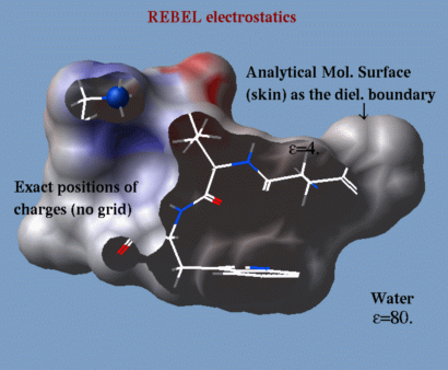
|
- electroMethod = "boundary element";
- dielConst (the default is usually OK);
- dielConstExtern (the default is usually OK);
- set charge as_ r_Charge (modify charges if you like);
- make boundary (if you want to make several evaluations of energy or Potential( ) with the same boundary. The "boundary" parameters depend only on conformation and do NOT depend on charges. You can redefine charges afterwards and get a corrects energy evaluation);
- delete boundary (if you do not need it);
- show energy (make sure the "el" term is on);
- Potential ( as_targets as_charges) (if the boundary exists, returns potentials from charges at the target atoms);
- color grob potential (create graphics object, say, with make grob skin actually it can be any grob and color it by the REBEL potential);
electroMethod = 4
show energy "el"
Rarray( a_//* )
!- real number may exist in the ICM-shell as a named variable or a constant (e.g. 12.3, 2.0, -4.501 ). There are a number of predefined real variables. Reals may be mentioned in arithmetic expressions, commands and functions.
Examples:
 a = -1.2
 b = Abs(Sin( 2.3 * a - 3.0 / a))
!- regularization procedure for fitting a protein model with the ideal covalent geometry of residues (as represented in the icm.res residue library) to the atom positions of a target PDB structure (usually provided by X-ray crystallography or NMR). Regularization is required because the experimentally determined PDB-structures often lack hydrogen atoms and positional errors may result in the unrealistic van der Waals energy even if these structures were energetically refined (since the refinement of the crystallographic structures typically ignores hydrogen atoms and employs different force fields). The following steps are required to create the regularized and energy refined ICM-model of an experimental structure:
- an extended all-atom model of a particular protein is generated with regular geometry characteristics (see the build command and the IcmSequence function);
- the non-hydrogen atoms in the model are assigned to the equivalent atoms in the model (see set tether);
- the regularized structure is built starting from the N-terminus by adding atoms one-by-one (see minimize tether);
- methyl groups are rotated to reduce van-der-Waals clashes;
- combined geometry and energy function is optimized;
- polar hydrogen positions are adjusted;
- optionally the model may be additionally minimized, now without tethers to observe a "stability" of the model in the local energy minimum.
!- residue a chemical building block or complete chemical compound, usually an amino-acid residue. The ICM hierarchy: atom -> residue -> molecule -> object. Individual small molecules may contain only one residue. Residues are described in the icm.res file. You may create your own residues with the write library command. Residues can be selected with the ICM-selection expression (e.g. a_/ala, a_/15, a_/15:20, a_/"RDGE" etc.), labeled with the display residue label rs_ command, by double clicking with the right mouse button, via a pop-up menu, or from the GUI menu.
!- rgb red-green-blue. It is of interest, that the combination of these three can produce any other color. In addition, this is the name of the SGI image format used in the ICM commands write image and display movie . ICM also generates the fourth channel on top of the RGB information. This fourth number is called alpha-channel and generates the opacity index for each pixel of the image. This information is interpreted by a number of applications, i.e. the IRIX showcase and dmconvert (the SGI moviemaker). See also tif, targa, postscript.
!- ribbon
|
a graphical representation of a polypeptide chain backbone by a smooth
solid ribbon. DNA and RNA can be also displayed in a ribbon style.
There are three types of elements of the ribbon display depending on the secondary structure assigned to a given residue. |
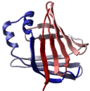
|
Residues marked as alpha-helices ('H') will be shown by a flat ribbon, those marked as beta-sheets ('E') will be flat ribbon with an arrow-head, and the rest will be shown by a cylindrical "worm". The ICM-shell parameter GRAPHICS.wormRadius defines its radius. Default ribbon colors are defined in the icm.clr file. Note that minor secondary structure elements like 3/10 helix ('G'), Pi-helix ('I') are colored by the corresponding colors ( the threetenRibbn and piRibbon parameters in the icm.clr file), 'Y' type is colored by the alphaRibbon color, and 'L','P' and 'B' (isolated beta-residue) residues are colored by the "betaRibbon" color. DNA and RNA ribbons are colored according to the base type: A-red, C-cyan, G-blue, T or U - gold. Preference ribbonStyle allows to display a simplified segment representation of the secondary structure elements instead of (or together with) the ribbon.
The DNA/RNA ribbons consists of two parts the backbone ribbon and the bases shown with the sticks and balls. To selectively display and undisplay the bases, you can do the following:
Example:
 read pdb "1dnk"         # contains 2 dna mol.
 display ribbon a_1.2,3  # both bases and backbone
 undisplay ribbon base a_1.2    # bases disappear
 display ribbon base only a_1.2 # only bases
 display ribbon a_1.2,3 yellow  # both bases and backbone
 color ribbon a_1.3 magenta     # the second chain backbone
 color ribbon a_1.2,3 bases     # default by base type
 cool a_  # cool is a rich macro. View the whole thing
!- script (or ICM script) means a collection of ICM commands stored in a file which can be called from ICM-shell.
Example:
call _demo_fold # find demo_fold file and start the script
!- sequence an ICM-shell object containing an amino-acid or DNA sequence. The ICM-shell is tuned to work with very large sets sets of millions of genomic sequences at once. To work with the sets larger than 2 Gigabytes in size use the 64-bit binary executable (it is standard on Cray and Dec, unavailable on Windows and optional on SGI). One can read a sequence from a sequence file in different formats, create it with the Sequence() function, make sequence command, or by assignment (e.g., aseq = bseq [2:18], new sequence aseq is a 2:18 fragment of sequence bseq). A valid amino-acid sequence contains an uppercase string of one-characters amino-acid names. Please distinguish this ICM-shell object from the "sequence" in the ICM-sequence file which contains detailed 3 (or 4)-character notations of residues from the icm residue library. One can concatenate two sequences ( seq1 // seq2 ) and extract a part of it ( seq[15:67] ). Sequence object may contain the secondary structure string (e.g. EEE___HHH_) of the same length as the sequence. It is automatically created by the make sequence command and the Sequence( ) function or can be directly set with the set sstructure command. If logical l_showSstructure is set to yes, the secondary structure string will be shown in alignments.
Examples:
 aseq=Sequence("ASSAARTYIP")
 read sequences "aa.seq"
 aseq[3:4]="WW"

 read object "crn"
 crn_seq = Sequence(a_/*)
Resetting sequence type
ICM is trying to guess sequence type. To set sequence type explicitly, use the set type [protein|nucleotide] command. E.g.
  a=Sequence("AAAATAAAA")
  set type a protein  # or if you change your mind
  set type a nucleotide
Properties of a sequence can be projected to an alignment in which the sequence participates with the Rarray( R_property,seq_,ali_,r_gapDefault ) function. The opposite action, i.e. projecting from alignment to a particular sequence can be achieved with another form of the Rarray function: Rarray( R_ali,ali_from,seq_|i_seqNumber )
!- segment an element of the simplified representation of a protein topology in terms of its secondary structure elements ( Abagyan and Maiorov, 1988). One element (referred to as a segment) is a vector of the best axis of the element. Loop segments are represented by a straight line between the end of the previous segment and the beginning of the next one. This representation can be used for a fold search through a library of precalculated segment descriptions of the protein topologies (foldbank.seg). See also ribbonStyle.
!- (ICM)-shell user-friendly, high-level command interpreter combined with a collection of tools allowing you to interact conveniently with the kernel of the ICM software.
!- skin a solid graphical representation of the molecular surface, also referred to as the Connolly surface. It is a smooth envelope touching the van der Waals surface of atoms as the solvent probe of the waterRadius size rolls over the molecule. "Skin" is important for analysis of recognition, electrostatics, energetics, ligand binding and protein cavities. The surface is calculated with a new fast analytical contour-buildup algorithm ( Totrov and Abagyan, 1996) and can be generated as a general graphics object with the make grob skin command. 'Skin' consists of three types of elements: convex spherical elements, concave spherical elements, and torus-shaped elements. ICM allows the calculation of the volume confined by the 'skin' and its surface area. In a general case skin is defined by two atom-selections:
- atoms the skin is calculated for
- atoms surrounding the atoms from the previous selection
 read object "complex"
 display a_//ca,c,n
 pocket = a_1//!h* & Sphere(a_2//!h*)
 display skin pocket a_1//!h* # 5A sphere around the second subunit
 set plane 2                  # or F2 : to avoid deletion of the previous patch
 display skin a_2//!h* a_2//!h* green # ignore everything but the second molecule
Colored molecular surface can be saved as:
- bitmap image (tif, targa, gif, postscript bitmap) ( write image "file")
- vectorized postscript containing triangles, not pixels ( write postscript "file")
- the skin can be converted into a uniform color grob ( make grob skin)
- the skin can be colored by potential and ( ( color grob potential try also: show dsRebel )
- Warning: make grob image does not generate correct normals because of a feature in OpenGL, however, this command works fine for molecular representations such as cpk , ribbon , xstick , etc.
ICM can also generate smooth gaussian surfaces with the following commands:
 make map potential Box( a_ 3. )   # build gaussian map
 make grob m_atoms solid exact 0.5 # contour it
 display g_atoms                   # display the envelope grob
!- smiles Simplified Molecular Input Line Entry Specification. The acronym introduced by David Weininger to represent chemical valence model by a string (e.g. CC=O). It can also be used as an exchange format for chemical data. The algorithm was published in 1988 and is described in detail at the WWW site of Daylight Chemical Information Systems, Inc.
See also the Smiles function and the build smiles command.
!- sln Sybyl line notation, a string representation of molecular structure similar to Smiles. The sln string is returned by the String( as_ sln ) function.
!- stack a set of conformations of a particular object. The stack can be just a place to store (with the store conf command) a number of complete descriptions of different conformations regardless of the way they have been created. The maximal number of stack conformations is determined by the mnconf parameter. The stack conformations can be created manually in the course of interactive procedure, or created automatically as a result of a montecarlo run. The energies of stack conformations can be shown with the show stack [all] command. The stack can be saved into a .cnf file, and you can also read stack. Stack in Biased Probability Monte Carlo procedure represents best energy representatives of different conformational families (see Abagyan and Argos, 1992). Measure of difference (or distance) is defined by the compare command and vicinity parameter. Stack can influence the search via the following variables: mnvisits, mnhighEnergy, mnreject, visitsAction, highEnergyAction and rejectAction .
See also:
- conf (has good examples),
- Table(stack) stack conformation parameters
- Iarray(stack) (the number of visits to each stack conformation).
- Nof (conf)
- load conf i
!- stick graphical representation of a covalent bond as a solid cylinder. Its radius is defined by the GRAPHICS.stickRadius ICM-shell variable.
!- string may exist in the ICM-shell as a named variable or a constant (e.g. "1crn", "A b\n c" ). There is a number of predefined string variables in the ICM-shell. You can concatenate strings ( "aaa" +"bbb" or "aaa" //"bbb" -> "aaabbb"), sum a string and a number ("aaa"+4.5 -> "aaa4.5" ), compare them ( if ( s_pdbDir == "/data/pdb/", or if ( s1 > s2 ) ). Strings may be used in arithmetic expressions, commands and functions.
Examples:
 s  = "1crn"
 s1 = s1 + ".brk"
 if (s != "2ins") print "wrong protein"
!- structure factor (factor) a named ICM-shell table containing information about reflections. A structure factor table header may contain maximal absolute values of h k and l.
#>I igd.HKL
 31 36 37
It will be calculated on the fly if absent and is important for Fourier transformation. You may also have any number of additional members in the header section for your convenience. For example, real values for the minimal and maximal resolution, etc.
The "column" part of a table contains mandatory integer arrays of h,k and l. Some of the other arrays with fixed names may be necessary for specific operations. They are:
- fo : real array of observed amplitudes (used by the "xr" term)
- fc : real array of calculated amplitudes. They are added and updated automatically by the "xr" term calculations.
- ac and bc : real array of Real and Imaginary components of calculated structure factors. ac and bc may be read from a file, calculated in the ICM-session, and/or added and updated automatically by the "xr" term calculations. These two arrays are used as the input arrays for the make map factor command.
- w : real array of weights of individual reflections which are used if defined in the "xr" term calculations. Note, that multiplicity will be automatically taken into account, do not multiply your weights by it to avoid double counting.
- free : integer array of 0 and non-zeros to mark reflections for R-free calculations. Reflections marked with non-zeros will not be used in the "xr" term calculations. They will be used instead by the Rfree( T_factor) function.
One can add any number of additional arrays to the factor-table. Of course, the table can be read, written, sorted, shown, etc. You may also use powerful table arithmetics and expressions to generate new columns and specify subsets.
Examples:
                                   # new columns
 group table append F Sqrt(F.ac*F.ac+F.bc*F.bc) \
       "fc" Atan2(F.bc,F.ac) "ph_calc"

 F.ac = (2*F.fo-F.fc)*Cos(F.ph_calc)
 F.bc = (2*F.fo-F.fc)*Sin(F.ph_calc)
 make map factor F    # 2Fo - Fc map is ready

 F1= F.fc > 1. # another table of strong reflections
 F2= F.h < 20 & F.k < 30 & F.l < 20 # another subset
See also:
How to manipulate with structure factors
The command word "factor" serves to read/write the XPLOR formatted structure-factor-files.
!- surface area in the ICM-shell means a solvent-accessible surface (center of water-sphere). Important: Do not confuse this surface with the molecular or Connolly surface which is referred to as skin . (see also Acc function, Area function, display skin,display surface, show area surface,show area skin, show volume surface "sf" term ).
Important: There are two ways to calculate the surface area: via the show area surface or the show energy "sf" commands. In both cases individual atomic accessibilities are calculated and assigned to individual atoms. These accessibilities can be shown with the show as_ command, or can be accessed with the Area( as_) function. However, the two commands use different atomic radii:
- show area surface
- uses van der Waals radii as defined in the icm.vwt file
- calculates areas for all atoms including hydrogens
- show energy "sf"
- uses special radii designed for calculations of the solvation energy. The radii are defined in the icm.hdt file ;
- employs a united atom model, in which hydrogens are ignored and radii increased accordingly;
- calculates areas only for non-hydrogen atoms, ignores hydrogens.
Examples:
                    # dipeptide
 build string "se nter ala his cooh"
                    # fill out individual accessibilities
                    # (incl. hydrogens)
 show area surface  # takes all atoms w. vdWaals radii into account
 show a_//*         # look at the accessibilities
 show Area(a_//n*)  # extract atomic accessibilities for all nitrogens
#
 show energy "sf"   # only heavy atom accessibilities used in energy calc.
 show a_//*         # look at these new accessibilities
 show Area(a_//n*)  # "energy" accessibilities for nitrogens
| Prev E H | Home Up | Next T |