| Prev | 2.21 Functions | Next |
[ Abs | Acc | Acos | Acosh | _Align | Angle | Area | Areacontactmatrix | Asin | Asinh | Ask | Atan | Atan2 | Atanh | Atom | Augment | Axis | Bfactor | Boltzmann | Box | Bracket | Cad | Ceil | Cell | Charge | Cluster | _Color | Consensus | Corr | Cos | Cosh | Count | Date | Deletion | Det | Disgeo | Distance | Eigen | Energy | Error | Exist | Existenv | Extension | Exp | Field | Fielduser | File | _Find | Floor | Getenv | Gradient | _Grob | Group | Histogram | Iarray | Iarrayatoms | nvis | IcmSequence | Index | _Indexx | Insertion | Info | Integer | Integral | Interrupt | Label | Length | LinearFit | Link | Log | Map | Mass | Matrix | Max | MaxHKL | Mean | Min | Money | Mod | Mol | Name | Namex | Next | Nextcovalentneighbors | Nof | Norm | Obj | Occupancy | Path | Parray | Pattern | Pi | Potential | Power | Probability | Profile | Putenv | Radius | Random | Rarray | Real | Remainder | Replace | Res | Resali | Resolution | Rfactor | Rfree | Rmsd | Rot | Sarray | Score | Select | Sequence | reversecompdnaseq | Sign | Sin | Sinh | Site | Smiles | Smooth | Split | Sql | Sqrt | Sphere | _Split | Srmsd | String | Sstructure | Sum | Symgroup | Table | alitable | Tablestack | Tan | Tanh | Tensor | Temperature | Time | Tolower | Torsion | Toupper | Tr123 | Tr321 | Trace | Trans | Transpose | Trim | Turn | Type | Unix | Value | Vector | Version | Volume | View | Warning | Xyz ]
ICM-shell functions are an important part of the ICM-shell environment. They have the following general format: FunctionName ( arg1, arg2, ... ) and return an ICM-shell object of one of the following types: integer, real, string, logical, iarray, rarray, sarray, matrix, sequence, profile, alignments, maps, graphics objects (grob) and selections.The order of the function arguments is fixed in contrast to that of commands. The same function may perform different operations and return ICM-shell constants of different type depending on the arguments types and order. ICM-shell objects returned by functions have no names, they may be parts of algebraic expressions and should be formally considered as 'constants'. Individual 'constants' or expressions can be assigned to a named variable. Function names always start with a capital letter. Example:
show Mean(Random(1.,3.,10))
2.21.1 Abs | [Top] |
Abs ( real ) - returns real absolute value.
Abs ( integer ) - returns integer absolute value.
Abs ( rarray ) - returns rarray of absolute values.
Abs ( iarray ) - returns iarray of absolute values.
Examples:
 a=Abs(-5.)                 # a=5.
 print Abs({-2.,0.1,-3.})   # prints rarray {2., 0.1, 3.}
 if (Abs({-3, 1}=={3 1}) print "ok"
2.21.2 Acc | [Top] |
Acc ( rs_ , [ r_Threshold ] )
- returns residue selection, containing a subset of specified residues `rs_ for which the ratio of their current accessible surface to the standard exposed surface is greater than the specified or default threshold (0.25 by default). ICM stores the table of standard residue accessibilities in an unfolded state calculated in the extended Gly-X-Gly dipeptide for all amino acid residue types. It can be displayed by the show residue type command, or by calling function Area( s_residueName ), and the numbers may be modified in the icm.res file.
The actual solvent accessible surface, calculated by a fast dot-surface algorithm, is divided by the standard one and the residue gets selected if it is greater than the specified or default threshold. ( r_Threshold parameter is 0.25 by default).
Acc ( as_select, [ r_Threshold ] )
- returns atom selection, containing atoms with accessible surface divided by the total surface of the atomic sphere in a standard covalent environment greater than the specified or default threshold (0.1). Accessibility at this level does not make as much sense as at the residue level. The standard surface of the atom was determined for standard amino-acid residues. Note that hydrogens were NOT considered in this calculation. Therefore, to assign surface areas to the atoms use
show surface area a_//!h* a_//!h*
command or the
show energy "sf"
command.
You may later propagate the accessible atomic layer by applying Sphere( as_ , 1.1), where 1.1 is larger than a typical X-H distance but smaller than the distance between two heavy atoms. (the optimal r_Threshold at the atomic level used as the default is 0.1, note that it is different from the previous ).
Examples:
                                   # let us select interface residues
 read object s_icmhome+"complex"
                                   # display all surface residues
 show surface area
 display Acc( a_/* )
                                   # now let us show the interface residues
 display a_1,2
 color a_1 yellow
 color a_2 blue
 show surface area a_1 a_1         # calculate surface of
                                   # the first molecule only

                                   # select interface residues
                                   # of the first molecule
 color red Sphere(a_2/* a_1/* 4.) & Acc(a_1/*)

 read object "crn"
 show energy "sf"
 display
 display cpk Acc(a_//* 0.1)   # display accessible atoms

 show surface area            # prior to invoking Acc function
                              # surface area should be calculated
 color Acc(a_/*) red          # color residues with relative
                              # accessibility > 25% red
2.21.3 Acos | [Top] |
Acos ( real | integer ) - returns the real arccosine of its real or integer argument.
Acos ( rarray ) - returns the rarray of arccosines of rarray elements.
Examples:
 print Acos(1.)               # equal to 0.
 print Acos(1)                # the same

 print Acos({-1., 0., 1.})    # returns {180. 90. 0.}
2.21.4 Acosh | [Top] |
Acosh ( real | integer ) - returns the real inverse hyperbolic cosine of its real or integer argument.
Acosh ( rarray ) - returns the rarray of inverse hyperbolic cosines of rarray elements.
Examples:
 print Acosh(1.)               # returns 0
 print Acosh(1)                # the same

 print Acosh({1., 10., 100.})  # returns {0., 2.993223, 5.298292}
2.21.5 Align | [Top] |
Align ( [ sequence1, sequence2 [{ area | distance | superimpose } [ i_window] [ r_seq_weight]] ] ) - returns ZEGA- alignment . If no arguments are given, the function aligns the first two sequences in the sequence list.
Returned variables:
- i_out - the number of identical residues in the alingment
- r_out - contains Log( Probability_of_structural_dissimilarity ) only for pairwise alignments
- r_2out - percent identity of the alignment.
Simple pairwise sequence alignment
Align( )
Align( seq1 seq2 ) - returns an alignment. The alignMethod preference allows you to perform two types of pairwise sequence alignments: "ZEGA" and "H-align". If you skip the arguments, the first two sequence are aligned.
Example:
   read sequences s_icmhome+"sh3.seq" # read 3 sequences
   print Align(Fyn,Spec)              # align two of them
   Align( )                           # the first two
   a=Align( sequence[1] sequence[3] ) # 1st and 3rd
   if(r_out > 5.) print "Sequences are struct. related"
Aligning with custom residue weights or weights according to surface accessible area
Align( seq1 seq2 area )
Option area will use relative residue accessibilities to weight the residue-residue substitution values in the course of the alignment (see also accFunction ).
The weights must be positive and less than 2.37 . Try to be around or less than 1. since relative accessibilities are always in [0.,1.] range. Values larger than 2.37 do not work well anyway with the existing alignment matrices and gap parameters. Use the Trim function to adjust the values, e.g. Trim( myweights , 0.1,2.3 ) ).
E.g.
 read pdb "1lbd"
 show surface area
 make sequence
  Info> sequence  1lbd_m  extracted
 1lbd_m                       # see the relative areas
 read pdb sequence "1fm6.a/"  # does not have areas
 Info> 1 sequence 1fm6_a  read from /data/pdb/fm/pdb1fm6.ent.Z
 ali3d = Align( 1lbd_m 1fm6_a area )
This can also be used to assign custom weights with the following commands
 set area seq1 R_weights  # must be > 0. and less than 2.37
 Align( seq1 seq2 area )
Introducing positional terms into the alignment score.
Align( seq1 seq2 M_positionalScores )
If sequence similarity is in the "twilight zone" and the alignment is not obvious, the regular comp_matrix{residue substitution matrix} is not sufficient to produce a correct alignment and additional help is needed. This help may come in a form of the positional information, e.g. histidine 55 in the first sequence must align with histidine 36 in the second sequence, or the predicted alpha-helix in the first sequence preferably aligns with alpha-helix in the second one.
In this case you can prepare a matrix of extra scores for each pair of positions in two sequences, e.g.
 seq1 = Sequence("WEARSLTTGETGYIPSA")
 seq2 = Sequence("WKVEVNDRQGFVPAAY")
 Align()
 # Consensus   W.#.  .~~.~G%#P^
           WEARSLTTGETGYIPS--
           WKVE--VNDRQGFVPAAY
 m = Matrix(17,16,0.)
 m[10,4] = 3. # reward alignment of E in seq1[10]  and E in seq2[4]
 Align(seq1 seq2 m )
 # Consensus   W.#      E    ~G%#P^
           WEARSLTTGE----TGYIPS--
           WKV------EVNDRQGFVPAAY
The alignSSmacro shows a more elaborate example in which extra scores are prepared to encourage alignments of the same secondary structure elements.
Warning. The alignment procedure is very subtle. Avoid values comparable with gap opening penalty.
Local structural alignment
Two types of structural alignments or mixed sequence/structural alignments can be performed with the Align function.
Align( seq_1 seq_2 distance [ i_window ] [ r_seq_weight ] ) - performs local structural alignment, using distance RMSD as structural fitness criterion. The RMSD is calculated in a window i_window and the dynamic programming algorithm combines structural scores with sequence alignment scores if r_seq_weight > 0.,
Align( seq_1 seq_2 superimpose [ i_window ] [ r_seq_weight ] ) - performs local structural alignment, using superposition followed by coordinate RMSD calculation as structural fitness criterion. The RMSD is calculated in a window i_window and the dynamic programming algorithm combines structural scores with sequence alignment scores if r_seq_weight > 0.,
In both cases the function uses the dynamic algorithm to find the alignment of the locally structurally similar backbone conformations.
The alignment based on optimal structural superposition of two 3D structures may be different from purely sequence alignment
Preconditions:
- sequences must be linked to 3D molecules to access the coordinate information;
- two 3D structures must have a superimposable subsets
Extracting pairwise alignment sequences from a multiple alignment
Align ( ali_, seq_1, seq_2 ) - returns a pairwise sub- alignment of the input alignment ali_, reorders of sequences in the alignment according to the order of arguments.
Extracting a multiple alignment of a subset of sequences from a multiple alignment
Align ( ali_, I_seqNumbers ) - returns a reordered and/or partial alignment . Sequences are taken in the order specified in I_seqNumbers.
Examples:
             # 14 sequences
 read alignment msf s_icmhome + "azurins"
             # extract a pairwise alignment by names
 aa = Align(azurins,Azu2_Metj,Azur_Alcde)
             # reordered sub-alignment extracted by numbers
 bb = Align(azurins,{2 5 3 4 10 11 12})
Resorting alignment in the order of sequence input with the Align ( ali_, I_seqNumbers ) function.
Load the following macro and apply it to your alignment. Example:
 macro reorderAlignmentSeq( ali_ )
  nn=Name(ali_)  # names in the alignment order
  ii=Iarray(Nof(nn))
  j=0
  for i=1,Nof(sequence)  # the original order
   ipos = Index( nn, Name(sequence[i] ) )
   if ipos >0 then
     j=j+1
     ii[j] = ipos
   endif
  endfor
  ali_new = Align( ali_ ii )
  keep ali_new
 endmacro
Deriving an alignment from tethers between two 3D objects
Align ( ms_ ) - returns alignment between sequences of the specified molecule and the template molecule to which it is tethered. The alignment is deduced from the tethers imposed.
This function may be used to save the alignment after interactive editing.
Example:
 build string "se ala his leu gly trp ala" "a"  # obj. a
 build string "se his val gly trp gly ala" "b"  # obj. b
 set tether a_2./1:3 a_1./2:4 align                 # impose tethers
 show Align(a_2.1)         # derive alignment from tethers
 write Align(a_2.1) "aa"   # save it to a file
2.21.6 Angle | [Top] |
Angle ( as_atom ) - returns the planar angle defined by the specified atom and two previous atoms in the ICM-tree. For example, Angle(a_/5/c) is defined by C-Ca-N atoms of the 5-th residue. You may type:
print Angle( # and then click the atom of interest.
Angle ( as_atom1 , as_atom2 , as_atom3 ) - returns the planar angle defined by three atoms.
Angle ( R_3point1 , R_3point2 , R_3point3 ) - returns the planar angle defined by the three points.
Angle ( R_vector1 , R_vector2 ) - returns the planar angle between the two vectors.
Examples:
 d=Angle( a_/4/c )                         # d equals N-Ca-C angle
 print Angle( a_/4/ca a_/5/ca a_/6/ca )    # virtual Ca-Ca-Ca planar angle
2.21.7 Area | [Top] |
Area ( grob ) - returns real surface area of a solid graphics object.
See also: the Volume( grob ) function, the split command and How to display and characterize protein cavities section.
Area ( as_ ) - returns rarray of pre-calculated solvent accessible areas for selected atoms `as_ .
Area ( rs_ ) - returns rarray of pre-calculated solvent accessible areas for selected residues `rs_ . These accessibilities depend on conformation.
Area ( rs_ type ) - returns rarray of maximal standard solvent accessible areas for selected residues `rs_ . These accessibilities are calculated for each residue in standard extended conformation surrounded by Gly residues. Those accessibilities depend only on the sequence of the selected residues and do NOT depend on its conformation. To calculate normalized accessibilities, divide Area( rs_ ) by Area( rs_ type )
Example:
read object "1crn"
show surface area
a=Area(a_/* )      # absolute conformation dependent residue accessilities
b=Area(a_/* type ) # maximal residue accessilities in the extended conformation
c = a/b            # relative (normalized) accessibilities
2.21.8 Area contact matrix | [Top] |
Example:
 read object "crn"  # good old crambin
 s=String(Sequence(a_/A))
 PLOT.rainbowStyle="blue/rainbow/red"
 plot area Area(a_/A, a_/A) comment=s//s color={-50.,50.} \
    link transparent={0., 2.} ds

 read object "complex"
 plot area Area(a_1/A, a_2/A) grid color={-50.,50.} \
    link transparent={0., 2.} ds
Area ( string ) - returns the real value of solvent accessible area for the specified residue type in the standard "exposed" conformation.
Important : "pre-calculated" above means that before invoking this function, you should calculate the surface by show area surface , show area skin or show energy "sf" commands.
Examples:
 build                   # build a molecule according to the sequence
                         # from file def.se (default)
 show area surface       # calculate surface area
 a = Area(a_//o*)        # individual accessibilities of oxygens

 stdarea = Area("lys")   # standard accessibility of lysine

# More curious example
 read object "crn"
 show energy "sf"        # calculate the surface energy contribution
                         # (hence, the accessibilities are
                         # also calculated)

 assign sstructure a_/* "_"
                         # remove current secondary structure assignment
                         # for tube representation
 display ribbon
                         # calculate smoothed relative accessibilities
                         # and color tube representation accordingly
 color ribbon a_/* Smooth(Area(a_/*)/Area(a_/* type) 5)
                         # plot residue accessibility profile
 plot Count(1 Nof(a_/*)) Smooth(Area(a_/*)/Area(a_/* type) 5) display
See also:
Acc( )
function.
2.21.9 Asin | [Top] |
Asin ( real | integer)
- returns the real arcsine of its real or integer argument.
Asin ( rarray )
- returns the rarray of arcsines of rarray elements.
Examples:
 print Asin(1.)               # equal to 90 degrees
 print Asin(1)                # the same

 print Asin({-1., 0., 1.})    # returns {-90., 0., 90.}
2.21.10 Asinh | [Top] |
Asinh ( real)
- returns the real inverse hyperbolic sine of its real argument.
Asinh ( rarray)
- returns the rarray of inverse hyperbolic sines of rarray elements.
Examples:
 print Asinh(1.)               # returns 0.881374
 print Asinh(1)                # the same

 print Asinh({-1., 0., 1.})    # returns {-0.881374, 0., 0.881374}
2.21.11 Ask | [Top] |
Ask( s_prompt, i_default )
- returns entered integer or default.
Ask ( s_prompt, r_default )
- returns entered real or default.
Ask ( s_prompt, l_default )
- returns entered logical or default.
Ask ( s_prompt, s_default [simple] )
- returns entered string or default. Option simple suppressed interpretation of the input and makes quotation marks unnecessary.
Examples:
 windowSize=Ask("Enter window size",windowSize)
 s_mask=Ask("Enter alignment mask","xxx----xxx")

 grobName=Ask("Enter grob name","xxx")
 display $grobName

 show Ask("Enter string, it will be interpreted by ICM:", "")
          #e.g. Consensus( myAlignm )

 show Ask("Enter string:", "As Is",simple)
          #your input taken directly as a string
2.21.12 Atan | [Top] |
Atan ( real | integer )
- returns the real arctangent of its real or integer argument.
Atan ( rarray )
- returns the rarray of arctangents of rarray elements.
Examples:
 print Atan(1.)                    # equal to 45.
 print Atan(1)                     # the same.

 print Atan({-1., 0., 1.})         # returns {-45., 0., 45.}
2.21.13 Atan2 | [Top] |
Atan2 ( r_x, r_y )
- returns the real arctangent of r_y/r_x in the range -180. to 180. degrees using the signs of both arguments to determine the quadrant of the returned value.
Atan2 ( R_x R_y )
- returns the rarray of arctangents of R_y/R_x elements as described above.
Examples:
 print Atan2(1.,-1.)                        # equal to 135.
 print Atan2({-1., 0., 1.},{-0.3, 1., 0.3}) # returns phases {-106.7 0. 73.3}
2.21.14 Atanh | [Top] |
Atanh ( real )
- returns the real inverse hyperbolic tangent of its real argument.
Atanh ( rarray )
- returns the rarray of inverse hyperbolic tangents of rarray elements.
Examples:
 print Atanh(0.)                    # returns 0.
 print Atanh(1.)                    # returns error

 print Atanh({-0.9999, 0., .9999})  # returns { -4.951719, 0., -4.951719 }
2.21.15 Atom | [Top] |
Atom ( as_Obj_or_Mol_or_Res_selection )
- returns selection converted to the atomic level.
Atom ( vs_ )
- returns atom selection (i.e. selection of atomic level) to which the selected variables vs_ belong.
Examples:
 asel=Acc(a_2/his)             # select accessible His residues of
                               # the second molecule
 show Atom(asel)               # show atoms of these residues
 show Atom( v_//phi )          # carbonyl Cs
See also: the Res, Mol, adn Obj functions.
2.21.16 Augment | [Top] |
Augment( R_12transformationVector )
- rearranges the transformation vector into an augmented affine 4x4 space transformation matrix .
The augmented matrix can be presented as
 a1  a2  a3  | a4
 a5  a6  a7  | a8
 a9  a10 a11 | a12
 ------------+----
 0.  0.  0.  | 1.
where {a1,a2,...a12} is the R_12transformationVector . This matrix is convenient to use because it combines rotation and translation. To find the inverse transformation simply inverse the matrix:
 M_inv = Power(Augment(R_12direct),-1))
 R_12inv = Vector(M_inv)
To convert a 4x4 matrix back to a 12-transformation vector, use the Vector( M_4x4 ) function.
See also: Vector (the inverse function), symmetry transformations, and transformation vector.
Augment ( R_6Cell )
- returns 4x4 matrix of oblique transformation for given cell parameters {a b c alpha beta gamma}.
This matrix can be used to generate real coordinates from fractional coordinates. It also contains vectors A, B and C. See also an example.
Example:
 display a__crn.        # load and display crambin: P21 group
 obl = Augment(Cell( ))  # extract oblique matrix
 A = obl[1:3,1]         # vectors A, B, C
 B = obl[1:3,2]
 C = obl[1:3,3]
 g1=Grob("cell",Cell( )) # first cell
 g2=g1+ (-A)            # second cell
 display g1 g2
Augment( R_3Vector ) - appends 1. to a 3D vector x,y,z (resulting in x,y,z,1. ) to allow direct arithmetics with augmented 4x4 space transformation matrixes.
Augment( M_XYZblock ) - adds 1.,1.,..1. column to the Nx3 matrix of with x,y,z coordinates to allow direct arithmetics with augmented 4x4 space transformation matrixes.
2.21.17 Axis | [Top] |
Axis( { M_33Rot | R_12transformation } )
- returns rarray with x,y,z components of the normalized rotation/screw axis vector. Additional information calculated and returned by the function:
See also: How to find and display rotation/screw transformation axis
2.21.18 Bfactor | [Top] |
Bfactor ( [ as_ | rs_ ] [ simple ] ) - returns rarray of b-factors for the specified selection of atoms or residues. If selection of residue level is given, the average residue b-factors are returned. B-factors can also be shown with the command show pdb.
Option simple returns a normalized b-factor. This option is possible for X-ray objects containing b-factor information. The read pdb command calculates the average B-factor for all non-water atoms. The normalized B-factor is calculated as (b-b_av)/b_av . This is preferable for coloring ribbons by B-factor since these numbers only depend on the ratios to the average. We recommend to use the following commands to color by b-factor:
 color ribbon a_/ Trim(Bfactor( a_/ simple ),-0.5,3.)//-0.5//3. # or
 color a_// Trim(Bfactor( a_// simple ),-0.5,3.)//-0.5//3.  # for atoms
This scheme will give you a full sense of how bad a particular part of the structure is.
See also: set bfactor.
Examples:
 avB=Min(Bfactor(a_//ca))     # minimal B-factor of Ca-atoms
 show Bfactor(a_//!h*)        # array of B-factors of heavy atoms
 color a_//* Bfactor(a_//*)   # color previously displayed atoms
                              # according to their B-factor
 color ribbon a_/A Bfactor(a_/A) # color the whole residue by mean B-fac.
2.21.19 Boltzmann | [Top] |
Example:
deltaE = Boltzmann*temperature # energy
2.21.20 Box | [Top] |
Box ( ) - returns the 6- rarray with {Xmin ,Ymin ,Zmin ,Xmax ,Ymax ,Zmax } parameters of the graphics box as defined on the screen.
Box ( center ) - returns the 6- rarray with Xcenter,Ycenter,Zcenter,Xsize,Ysize,Zsize parameters of the graphics box as defined on the screen.
Box ( as_ [ r_margin ] ) - returns the 6- rarray with Xmin,Ymin,Zmin,Xmax,Ymax,Zmax parameters of the box surrounding the selected atoms. The boundaries are expanded by r_margin (default: 0.0 ).
Examples:
 build string "se ala his"  # a peptide
 display box Box(a_/2 1.2)  # surround the a_/2 by a box with 1.2A margin
 color a_//* & Box( )
Box ( { g_ | m_ } [ r_margin ] )
- returns the 6- rarray with Xmin,Ymin,Zmin,Xmax,Ymax,Zmax parameters of the box surrounding the selected grob or map. The boundaries are expanded by r_margin (default: 0.0 ).
2.21.21 Bracket | [Top] |
Bracket ( m_grid [ r_vmin r_vmax ] )
- returns the truncated map . The map will be truncated by value. The values beyond r_vmin and r_vmax will be set to r_vmin and r_vmax respectively.
Bracket ( m_grid [ R_6box ] )
- returns the modified map . All the values beyond the specified box will be set to zero. Example:
 make map potential "gh,gc,gb,ge,gs" a_1 Box()
 m_ge = Bracket(m_ge, Box( a_1/15:18,33:47 )) # redefine m_ge
See also: Rmsd( map ) and Mean( map ), Min( map ), Max( map ) functions.
2.21.22 Cad | [Top] |
Cad can measure the geometrical difference between two conformations in several different ways:
- between two conformations of the same protein based on full atom residue-residue contact area calculation, Cad(..)
- between two conformations of the same protein based on Cbeta-Cbeta distance evaluation (`Cad1{Cad}(.. distance ) .ICM uses an empirically derived ContactStrength( Cb-distance ) function.
- between two homologous structures based preservation of the residue contacts through the alignment ( Cad (.. alignment )) . The contact strength in this case is also derived from the interresidue distances.
2.21.22.1 Comparing two conformations of the same molecule via residue-residue contact conservation. | [Top] |
- returns the real contact area difference measure (described in Abagyan and Totrov, 1997) between two conformations A and B of the same set of residue pairs from two different objects. The set of residue pairs in each object (A or B) can be defined in two ways:
- by a single selection rs_A1 : all pairs between selected residues (is equivalent to rs_A1 rs_A1 )
- by two residue selections rs_A1 rs_A2: cross pairs between two sets of selected residues (e.g. the contacts between two subunits)
The whole matrix of contact area differences is returned in M_out . This matrix can be nicely plotted with the plot area M_out number .. command (see example). The full matrix can also be used to calculate the residue profile of the differences.
The table of the pairwise contact area differences is written to the s_out string which can later be read into a proper table via: read column group name="aa" input=s_out and sorted by the area (see below).
See also Area() function which calculates absolute residue-residue contact areas.
Options:
- distance option allows to compare approximations of the inter-residue contact areas by the Ca and Cbeta positions. This allows to calculated deformations between two homologous proteins which is not possible in the default mode in which two chemically identical molecules are compared. The residue pairs in two homologues are equivalenced according to the alignments linked to the molecules. Residues deleted in a homologue are considered to have zero contact.
Examples:
# Ab initio structure prediction, Overall models by homology
   read pdb "cnf1"   # one conformation of a protein
   read pdb "cnf2"   # another conformation of the same protein
   show 1.8*Cad(a_1. a_2.)   # CAD=0. - identical; =100. different
   show 1.8*Cad(a_1.1 a_2.1) # CAD between the 1st molecules (domains)
   show 1.8*Cad(a_1.1/2:10 a_2.1/2:10) # CAD in a window
   PLOT.rainbowStyle = 2
   plot area grid M_out comment=String(Sequence(a_1,2.1)) link display

# Loop prediction: 0% - identical; ~100% totally different
#    CAD for loop 10:20 and its interactions with the environment
   show 1.8*Cad(a_1.1/10:20 a_1.1/* a_2.1/10:20 a_2.1/*)
#    CAD for loop 10:20 itself
   show 1.8*Cad(a_1.1/10:20 a_1.1/10:20 a_2.1/10:20 a_2.1/10:20)

# Evaluation of docking solutions: 0% - identical; 100% totally different
   read pdb "expr"   # one conformation of a complex
   read pdb "pred"   # another conformation of the same complex
   show Cad(a_1.1 a_1.2 a_2.1 a_2.2)  # CAD between two docking solutions
#
# ANOTHER EXAMPLE: the most changed contacts
   read object "crn"
   copy a_ "crn2"
   randomize v_ 5.
   Cad(a_1. a_2.)
   show s_out
   read column group input= s_out name="cont"
   sort cont.1
   show cont
# the table looks like this (the diffs can be both + and -):
#>T cont
#>-1-----------2-----------3----------
   -39.        a_crn.m/38  a_crn.m/1
   -36.4       a_crn.m/46  a_crn.m/4
   -32.1       a_crn.m/46  a_crn.m/5
   -29.8       a_crn.m/30  a_crn.m/9
   -25.2       a_crn.m/37  a_crn.m/1
...
   42.5        a_crn.m/43  a_crn.m/5
   45.1        a_crn.m/44  a_crn.m/6
   45.2        a_crn.m/43  a_crn.m/6
   55.3        a_crn.m/46  a_crn.m/7
   56.         a_crn.m/45  a_crn.m/7
2.21.22.2 Comparing two different, but structurally homologues proteins, via residue-residue contact conservation. | [Top] |
2.21.23 Ceil | [Top] |
Ceil ( r_real [ r_base] )
- returns the smallest real multiple of r_base exceeding r_real.
Ceil ( R_real [ r_base] )
- returns the rarray of the smallest multiples of r_base exceeding components of the input array R_real. Default r_base= 1.0 .
See also: Floor( ).
2.21.24 Cell | [Top] |
Cell ( { os_ | m_map } )
- returns the rarray with 6 cell parameters {a,b,c,alpha,beta,gamma} which were assigned to the object or the map.
2.21.25 Charge | [Top] |
Charges can also be shown with a regular show as_select command.
Charge ( { os_ | ms_ | rs_ | as_ } [ formal | mmff ] )
- returns rarray of elementary or total charges depending on the selection level.
- formal : return formal charges
- mmff : return formal charges calculated according to mmff atom types and rules. Note: do not confuse this option with a function to return the mmff charges.
Examples:
 buildpep "ala his glu lys arg asp"
 show Charge(a_1)      # charge per molecule
 show Charge( a_1/* )  # charge per residue
 show Charge( a_1//* ) # charge per atom

 avC=Charge(a_/15)        # total electric charge of 15th residue
 avC=Sum(Charge(a_/15/*)) # another way to calculate it
 show Charge(a_//o*)      # array of oxygen charges

# to return mmff charges:
 set type mmff
 set charge mmff
 Charge( a_//* )

# to return total charges per molecular object:
 read mol s_icmhome+"ex_mol.mol"
 set type mmff
 set charge mmff
 Charge( a_*. )
See also: set charge.
2.21.26 Cluster | [Top] |
function returns iarray of cluster numbers for each or N points.
The input to the first function is an array of M nearest neighbors (defined by the second argument i_M_totalNofNearNeighbors) for each of N points. For example for an array for 5 points, and i_M_totalNofNearNeighbors = 3 it can be an array like this: {3,4,5, 1,3,4 1,2,5 2,3,5 1,2,3} . The points will be grouped into the same cluster if the number of neighbors they share is larger or equal than i_minNofCommonNeighbors . This clustering algorithm is adaptive to the cluster density and does not depend on absolute distance threshold. In other words it will identify both very sparse clusters and very dense ones. The nearest neighbor array can be calculated by the with the Link ( I_bitkeys , nBits, nNearestNeighbors ) function.
Cluster( M_NxNdist r_maxDist ) ⇒ I_N_clusterNumbers
This function identifies the i_totalNofNeighbors nearest neighbors from the full distance matrix M_NxNdist for each point and assembles points sharing the specified number of common neighbors in clusters.
All singlets (a single item not in any cluster) are placed in a special cluster number 0 . Other items are assigned to a cluster starting from 1.
Example with a distance matrix:
# let us make a distance matrix D
# we will cook it from 5 vectors {0. 0. 0.}
 m=Matrix(5,3)  # initialize 5 vectors
 m[2,1:3]={1. 0. 0.}   # v2
 m[3,1:3]={1. 1. 0.}   # v3
 m[4,1:3]={1. 1. 1.}   # v4
 m[5,1:3]={1. 0.1 0.1} # v5 close to v2

 D = Distance( m )  # 5x5 distance matrix created

 Cluster( D , 0.2 ) # v2 and v5 are assigned to cluster 1
 Cluster( D , 0.1 ) # radius too small. All items are singlets
 Cluster( D , 2.  ) # radius too large. All items are in cluster 1
2.21.27 Color | [Top] |
Color ( g_grob ) - returns matrix of RGB numbers for each vertex of the g_grob (dimensions: Nof ( g_grob),3).
See also: color g_ M_
Example:
 build string "se his"
 display xstick
 make grob image name="g_"
 display g_ only smooth
 M_clr = Color( g_ )
 for i=1,20    # shineStyle = "color" makes it disappear completely
   color g_ (1.-i/20.)*M_clr
 endfor
 color g_ M_clr
Color( background )
- returns rarray of three RGB components of the background color.
2.21.28 Consensus | [Top] |
- returns the string consensus of alignment ali_. The consensus characters are these: # hydrophobic; + RK; - DE; ^ ASGS; % FYW; ~ polar. In the selections by consensus a letter code (h,o,n,s,p,a) is used.
Consensus ( ali_ { i_seq | seq_ } )
- returns the string consensus of alignment ali_ as projected to the sequence.
Sequence can be specified by its order number in the alignment or by name.
Example displaying conserved residues:
 read alignment "sx"  # load alignment
 read pdb "x"         # structure
 display ribbon
        # multiply rs_ by a mask like "  A C   N  .."
 cnrv = a_/A & Replace(Consensus(sx cd59),"[.^~#]"," ")
 display cnrv red
 display residue label cnrv
2.21.29 Corr | [Top] |
Corr ( R_array1, R_array2 )
- returns the real value of the linear correlation coefficient. Probability of the null hypothesis of zero correlation is stored in r_out .
Examples:
 r=Corr(a,b)                   # two vectors a and b
 if (Abs(r_out) < 0.3) print "it is actually as good as no correlation"
See also: LinearFit( ) function.
2.21.30 Cos | [Top] |
Cos ( { r_Angle | i_Angle } )
- returns the real value of cosine of its real or integer argument.
Cos ( rarray )
- returns rarray of cosines of each component of the array.
Examples:
 show Cos(60.)                           # returns 0.5
 show Cos(60)                            # the same

 rho={3.2 1.4 2.3}                       # structure factors
 phi={60. 30. 180.}                      # phases
 show rho phi rho*Cos(phi) rho*Sin(phi)  # show in columns rho, phi,
                                         # Re, Im
2.21.31 Cosh | [Top] |
Cosh ( { r_Angle | i_Angle } ) - returns the real value of hyperbolic cosine of its real or integer argument. Cos(x)=0.5( eiz + e-iz )
Cosh ( rarray ) - returns rarray of hyperbolic cosines of each component of the array.
Examples:
 show Cosh(1.)                           # 1.543081
 show Cosh(1)                            # the same

 show Cosh({-1., 0., 1.})                # returns {1.543081, 1., 1.543081}
2.21.32 Count | [Top] |
Count ( [ i_Min, ] i_Max ) - returns iarray of numbers growing from i_Min to i_Max. The default value of i_Min is 1.
Examples:
 show Count(-2,1)         # returns {-2,-1,0,1}
 show Count(4)            # returns {1,2,3,4}
See also the Iarray( ).
Count ( array )
- returns iarray of numbers growing from 1 to the number of elements in the array.
2.21.33 Date | [Top] |
The allowed format specifications are the following:
| format | description | example |
|---|---|---|
| %D | day, say 1 or 12 or 30 | |
| %DD | day with compulsary two digits, say 01 03 12 etc. | |
| %M | month (say, 1) | |
| %MM | see above at %DD (say 01) | |
| %m | brief month (3 letter), say dec oct etc. | |
| %mm | full month (december) | |
| %Y | four letter year | |
| %YY - | ||
| %y | two letter year (damn with Y3K) | |
| %W | week day (say, Saturday) | |
| %w | three letter day (say, sat ) | |
| %z | time zone | |
| %HH | always aligned by two chars (03) | |
| %H | one or two chars | |
| %hh | the same with in pm/am style, | |
| %h | the same in pm/am style | |
| %pm | the string "pm" or "am", empty otherwise. | |
| %UU | minutes (say 01) | |
| %U | minutes (say 1, 12 ) | |
| %SS | seconds (say 04) | |
| %S | seconds (say 1, 4,12) |
Date()  # uses the default format
Date("%m %DD,%Y %h%pm") # today returns
 Oct 08,2002 5pm
2.21.34 Deletion | [Top] |
- returns the residue selection which flanks deletion points from the viewpoint of other sequences in the ali_Alignment. If argument seq_fromAli is given (it must be the name of a sequence from the alignment), all the other sequences in the alignment will be ignored and only the pairwise subalignment of rs_Fragment and seq_fromAli will be considered. The alignment must be linked to the object. With this function (see also Insertion function) one can easily and quickly visualize and/or extract all indels in the three-dimensional structure. The default i_addFlanks parameter is 1. String options:
- "all" (default: no string option) select deletions of all types
- "nter" select only N-terminal fragments
- "cter" select only C-terminal fragments
- "loop" select only the internal zones of deleted loops
See example coming with the Insertion( ) function description.
2.21.35 Det | [Top] |
Det ( matrix )
- returns a real determinant of specified square matrix.
Examples:
 a=Rot({0. 0. 1.}, 30.)     # Z-rotation matrix by 30 degrees
 print Det(a)               # naturally, it is equal to 1.
2.21.36 Disgeo | [Top] |
 group sequence se1 se2 se2 se4 mySeqs
 align mySeqs
 distMatr=Distances(mySeqs)
or any objects between which one can somehow define pairwise distances. Since principal coordinates are sorted according to their contribution to the distances and we can hardly visualize distributions in more than three dimensions, the first two or three coordinates give the best representation of how the points are spread in n-1 dimensions. Another application is restoring atomic coordinates from pairwise distances taken from NMR experiments.
Disgeo ( matrix )
- returns matrix [1:n,1:n] where the each row consists of n-1 coordinates of point [i] sorted according to the eigenvalue (hence, their importance). The first two columns, therefore, contain the two most significant coordinates (say X and Y) for each of n points. The last number in each row is the eigenvalue [i]. If distances are Euclidean, all the eigenvalues are positive or equal to zero. The eigenvalue represents the "principal coordinate" or "dimension" and the actual value is a fraction of data variation due to the this particular dimension. Negative eigenvalues represent "non-Euclidean error" in the initial distances.
Example:
 read sequences "zincFinger" # read sequences from the file,
 list sequences              # see them, then ...
 group sequence alZnFing     # group them, then ...
 align alZnFing              # align them, then ...
 a=Distance(alZnFing)        # a matrix of pairwise distances
 n=Nof(a)                    # number of points
 b=Disgeo(a)                 # calculate principal components
 corMat=b[1:n,1:n-1]         # coordinate matrix [n,n-1] of n points
 eigenV=b[1:n,n]             # vector with n sorted eigenvalues
 xplot= corMat[1:n,1]
 yplot= corMat[1:n,2]
 plot xplot yplot CIRCLE display # call plot a 2D distribution
2.21.37 Distance | [Top] |
[ Distanceiarray | Distancerarray | Distanceas_ | Distanceas_rarray | Distancematrix | DistanceTanimoto | Distancematrixtwosets | Distancetether | Distancedayhofffunction | Distancealignment | Distancetwoalignments ]
generic distance function. Calculates distances between two ICM-shell objects, bit-strings or molecular objects, or extracts distances from complex ICM-shell objects.2.21.37.1 Distance iarray | [Top] |
- returns the real sqrt of sum of (I1i -I2i )2 .
2.21.37.2 Distance rarray | [Top] |
2.21.37.3 Distance as_ | [Top] |
- Display your molecule
- type Dist , press TAB
- Ctrl-RightMB click on the atom you want (or double click for a residue) and press RETURN
2.21.37.4 Distance as_ rarray | [Top] |
2.21.37.5 Distance matrix | [Top] |
2.21.37.6 Tanimoto distance between two arrays of bit-strings | [Top] |
- returns the matrix of Tanimoto distances between two arrays of bit-strings. Each array of N-strings is represented by an iarray I_keys of N*( nBits/32 ) elements (e.g. if nBits is 32 , each integer represents 1 bit-string, if nBits i 64, I_keys1 has two integers for each bit string, etc.). The returned matrix dimensions are N1 x N2 . The distance is defined as 1. - similarity , where The Tanimoto similarity between bitstrings is defined as follows: The number of the on-bits in-common between two strings divided by the number of the on-bits in either bit-string.
You can provide a relative weight for each bit in a bit-string as a rarray R_weights. In this case the weighted Tanimoto distance is calculated as follows:
distWeighted = 1. - Sum( Wi_of_common_On_Bits ) / Sum( Wi_of_On_Bits )
With option simple the similarity calculation is modified so that the number of bits in common is divided by the number of bits in the second bit-string. For example:
Distance({3} {1} 32 simple ) # returns 0.
Distance({1} {3} 32 simple ) # returns 0.5
Example:
Distance({1 2 3},{1 2 3},32)
 #>M
 0. 1. 0.5
 1. 0. 0.5
 0.5 0.5 0.
The diagonal distances are 0; no bits are share between 1 (100..) and 2 (010..) (distance=1.) and
one of two bits is shared between 1 (100..) and 3 (110..).
Instead of the number of bits, one can provide the relative weights for each bit. The dimension of the bit-weight array then becomes the size of the bit-string. The weighted Tanimoto is calculated.
2.21.37.7 Distance matrix between two sets of coordinates | [Top] |
For example: Distance(Xyz(a_/1:5/ca) Xyz(a_/10:12/ca) returns a 5 by 3 matrix of distances between Ca-s of the two fragments.
2.21.37.8 Distance tether | [Top] |
- returns the real array of lengths of tethers for each selected atom or the default value ( -1. ). The default value can be set to any value. Tethers are assumed to be already set, see command set tether. Also note, that the expression Distance( as_out ) will give the same results if as_out selection was not changed by another operation; see also special selections.
Example:
read pdb "1crn" convert tether # keeps tethers to the pdb original deviations = Distance( a_//!h*,vt* , 9.9) perResDevs = Group( deviations, a_//!h*,vt* ,"max") # find max.devs per residue display ribbon color ribbon a_/* perResDevs # Another example Distance( a_//T ) # selects only tethered atoms #>R 1.677 1.493 1.386 1.435 1.645 1.570 2.165 1.399 |
|
2.21.37.9 Distance Dayhoff | [Top] |
- d1 = 1.0 - (nResidueIdentities/Min(Length(Seq1), Length(Seq2)) (d1 belongs to [0.,1.] range)
- if there is no identity option the distance is corrected: Distance(Seq1,Seq2) = DayhoffTransformation( d1 )
2.21.37.10 Distance alignment | [Top] |
1.-(nResidueIdentities-gapPenalty)/Min(Length(Seq1), Length(Seq2))where gapPenalty is 3 for each gap.
Without the fast option the distances are calculated based on comparison matrix and gap penalties. These distances are more sensitive but there is no simple mapping between them and percent identity based distances.
Example:
 read alignment msf "azurins"            # read azurins.msf
 NormCoord = Disgeo(Distance(azurins))   # 2D sequence diversity in
2.21.37.11 Distance two alignments | [Top] |
The distance is defined as a number of non-gap columns identical between two alignments.
Two different normalizations are available:
The default normalization is to the shorter alignment. ( Distance ( ali_1 ali_2 ) ). In this case the number of equivalent pairs is calculated and is divided by the total number of aligned pairs in the shorter alignment. This method detects alignment shifts but does not penalize un-alignment of previously aligned residue pairs. D = (La_min - N_commonPairs)/La_min In the following alignment the residue pairs which are aligned in both alignments are the same, therefore the distance is 0.
 show a1   # La1 = 3
 ABC---XYZ
 ABCDEF---
 show a2   # La2 = 6
 ABCXYZ
 ABCDEF
 Distance(a1,a2)   # a1 is a subalignment of a2, distance is 0.
 0.
exact option: normalization to the longer alignment. By longer we mean the larger number of aligned pairs regardless of alignment length (the latter includes gaps and ends). D = (La_max - N_commonPairs)/La_max Now in the above example, La_max = 6 , while N_commonPairs = 3, the distance is 0.5 (e.g. the alignments are 50% different).
Distance(a1,a2,exact) # returns 0.5 for the above a1 and a2
Example showing the influence of gap parameters:
 read sequence msf "azurins.msf"
 gapOpen =2.2
 a=Align(Azu2_Metj  Azup_Alcfa)   # the first alignment
 gapOpen =1.9                     # smaller gap penalty and ..
 b=Align(Azu2_Metj  Azup_Alcfa)   # the alignment changes
 show 100*Distance(a b )          # 20% difference
 show 100*Distance(a b exact )    # 21.7% difference
 show a b
2.21.38 Eigen | [Top] |
Eigen ( M_ )
- returns the square matrix of eigenvector columns of the input symmetric square matrix M_ . Eigenvalues sorted by their values are stored in the R_outrarray.
Example:
 A = Matrix(3, 3, 0.)      # create a zero square matrix...
 A[1:3,1] = {1.,-2.,-1.}   # and set its elements
 A[2,2] =  4.
 for i = 1, 3-1            # the matrix must be symmetric
   for j = i+1, 3
     A[i,j] = A[j,i]
   endfor
 endfor
 X = Eigen(A)              # calculate eigenvectors...
 V = R_out                 # and save eigenvalues in rarray V
 printf "eigenvalue 1 eigenvalue 2 eigenvalue 3\n"
 printf "%12.3f %12.3f %12.3f\n", V[1], V[2], V[3]
 printf "eigenvector1 eigenvector2 eigenvector3\n"
 for i = 1, 3
   printf "%12.3f %12.3f %12.3f\n", X[i,1], X[i,2], X[i,3]
 endfor
2.21.39 Energy | [Top] |
Energy ( string )
- returns the real sum of pre-calculated energy and penalty (i.e. geometrical restraints) terms specified by the string.
Important: the terms must be pre-calculated by invoking one of the following commands where energy is calculated at least once: show energy, minimize, ssearch command and montecarlo command.
Note:
- Allowed terms in the string are "vw,14,hb,el,to,af,bb,bs,cn,tz,rs,xr,sf";
- "func" stands for the total of all the terms, both energy and penalty;
- "ener" is only the energy part (i.e. "vw,14,hb,3l,to,af,bb,bs,sf" );
- "pnlt" is only the penalty part (i.e. "cn,tz,rs,xr" ).
- load conf and load frame commands fill out all the energy/penalty terms, which are stored in both stacks and movies (of course the values also depend on a set of free variables). You can get the energy/penalty terms of the loaded conformation without explicitly recalculating them.
Examples:
 build
 show energy
 print Energy("vw,14,hb,el,to")  # ECEPP energy

 read stack "f1"
 load conf 0
 print Energy("func")  # extract the best energy without recalculating it
Energy ( rs_ [ simple | base | s_energyTerms ] )
- calculates and returns residue energies in an ICM object. convert the object if is not of the ICM type. The energies are calculated according to the current energy terms , and also depend on the fixation of the object. Use unfix only V_//S to restore standard fixation.
This function can be used to evaluate normalized residue energies for standard amino-acids to detect local problems in a model.
For normalized energies, use the simple option. The base option just shifts the energy value to the mean energy for this residue type. If the simple or base terms are not used, the current energy terms are preserved. The energies calculated with the simple or base option are calculated with the "vw,14,hb,el,to,en,sf" terms. The terms are temporarily enforced as well as the vwMethod = 2 and vwSoftMaxEnergy values, so that the normalization performed with the simple option is always correct.
This function will calculate residue energies for all terms and set-ups with the following exceptions:
- electrostatic ( "el" ) term and electroMethod = "boundary element", "MIMEL", or "generalized Born"
The s_energyTerms argument allows to refine the energy terms dynamically (see example below).
Example:
  read pdb "1crn"
  delete a_W
  convert
  set terms "vw,14,hb,el,to,en,sf"
  group table t Energy( a_/A ) "energy" Label(a_/A ) "res"
  show t
  unfix V_//*
  group table tBondsAngles Energy( a_/A "bs,bb" ) "covalent" Label(a_/A ) "res"
  show tBondsAngles
See also: the calcEnergyStrain macro.
Energy ( conf i_confNumber)
- returns the table of all the energy components for the a given stack conformations.
The table has two arrays:
- sarray of the energy term names ( .hd ) and
- rarray of energy values for each energy term ( .ey ) and
Energy ({ stack | conf } )
- returns the rarray of total energies of stack conformations. Useful for comparison of spectra from different simulations.
Examples:
 set terms only "vw,14,hb,el,to"  # set energy terms
 show energy v_//xi*              # calculate energy with only
                                  # side chain torsions unfixed
           # energy depends on what variables are fixed since
           # interactions inside rigid bodies are not calculated,
           # and rigid body structure depends on variables

 a = Energy("vw,14")      # a is equal to the sum of two terms

 electroMethod="MIMEL"    # MIMEL electrostatics
 set terms only "el,sf"   # set energy terms
 show energy
 print Energy("ener")     # total energy
 print Energy("sf")       # only the surface part of the solvation energy
 print Energy("el")       # electrostatic energy
 print r_out              # electrostatic part of the solvation energy
2.21.40 Error | [Top] |
Error
- returns logical yes if there was an error in a previous command (not necessarily in the last one). After this call the internal error flag is reinstalled to no.
Error ( string )
- returns string with the last error message. It also returns integer code of the last error in your script in i_out . In contrast to the logical Error() function, here the internal error code is not reinstalled to 0, so that you can use it in expressions like if( Error ) print Error(string) .
Error ( i_error_or_warning_code ) ⇒ l Error ( number ) ⇒ s - returns logical yes if an error or warning with the specified code occurred previously in the script. This call also resets the flag (e.g. Error(415) ). This is convenient to track down certain warnings or errors in scripts (e.g. detecting if 'readpdb{read pdb} found certain problems).
Option number will return a string will previously set error and warning messages.
To clear all bits use the clear error command.
Examples:
 read pdb "1mng"  # this file contains strange 28-th residue
 if (Error) print "These alternative positions will kill me"

 read pdb "1abcd"  # file does not exist
 errorMessage = Error(string)
 ier = i_out
 if ier == 3102  print "What kind of name is that?"

 if=2
 if Error(2073) print "syntax error" # detect error [2073]
 read pdb "1mok"
 clear error
See also: errorAction , s_skipMessages , l_warn, Warning
Error ( r_x [ reverse ] )
- returns real complementary error function of real x : erfc(x)=1.-erf(x)) , defined as
(2/sqrt(pi)) integral{x to infinity} of exp(-t2) dt
or its inverse function if the option reverse is specified. It gives the probability of a normally distributed (with mean 0. and standard deviation 1./Sqrt(2.)) value to be larger than r_x or smaller than -r_x.
Examples:
 show 1.-Error(Sqrt(0.5)) # P of being inside +-sigma (about 68%)
 show Error(2.*Sqrt(0.5)) # P of being outside +- 2 sigma
Error ( R_x )
- returns rarray of erfc(x)=1.-erf(x)) functions for each element of the real array (see above).
Examples:
 x=Rarray(1000 0. 5. )
 plot display x Error(x ) {0. 5. 1. 1. 0. 1. 0.1 0.2 }
 plot display x Log(Error(x ),10.) {0. 5. 1. 1.}
       #NB: can be approximated by a parabola
       #to deduce the appr. inverse function.
       #Used for the Seq.ID probabilities.
2.21.41 Exist | [Top] |
Exist ( s_fileName ) - returns logical yes if the specified file or directory exists, no otherwise.
Exist ( key, s_keyName ) - returns logical yes if the specified keystoke has been previously defined. See also: set key command.
Exist ( object ) - returns logical yes if there is at least one molecular object in the shell, no otherwise.
Exist ( view ) - returns logical yes if the GL - graphics window is activated, no otherwise.
Exist ( gui ) - returns logical yes if the GRAPHICS USER INTERFACE menus is activated, no otherwise.
Examples:
 if (!Exist("/data/pdb/") then
   unix mkdir /data/pdb
 endif

 if(!Exist(key,"Ctrl-B")) set key "Ctrl-B" "l_easyRotate=!l_easyRotate"

 if !Exist(gui)  gui simple
2.21.42 Existenv | [Top] |
Existenv ( s_environmentName )
- returns logical yes if the specified named environment variable exists.
Example:
if(Existenv("ICMPDB")) s_pdb=Getenv("ICMPDB")
See also: Getenv( ), Putenv( ) .
2.21.43 Extension | [Top] |
Extension ( string [ dot ] )
- returns string which would be the extension if the string is a file name. Option dot indicates that the dot is excluded from the extension.
Extension ( sarray [ dot ] )
- returns sarray of extensions. Option dot indicates that the dot is excluded from the extensions.
Examples:
 print Extension("aaa.bbb.dd.eee")   # returns ".eee"
 show Extension({"aa.bb","122.22"} dot)         # returns {"bb","22"}
 read sarray "filelist"
 if (Extension(filelist[4])==".pdb") read pdb filelist[4]
2.21.44 Exp | [Top] |
Exp ( real )
- returns the real exponent.
Exp ( rarray )
- returns rarray of exponents of rarray components.
Exp ( matrix )
- returns matrix of exponents of matrix elements.
Examples:
 print Exp(deltaE/(Boltzmann*temperature))   # probability
 print Exp({1. 2.})                          # returns { E, E squared }
2.21.45 Field | [Top] |
Field ( s_ [ s_precedingString] i_fieldNumber [ s_fieldDelimiter] )
- returns the specified field. Parameter s_fieldDelimiter defines the separating characters (space and tabs by default). If the field number is less than zero or more than the actual number of fields in this string, the function returns an empty string.
The s_fieldDelimiter string
Single character delimiter can be specified directly, e.g.
 Field("a b c",3," ")  # space
 Field("a:b:c",3,":")  # colon
Alternative characters can be specified sequentially, e.g.
Field("a%b:c",3,"%:") # percent OR colon
Multiple occurence of a delimiting character can be specified by
repeating the same character two times, e.g.
 Field("a  b   c",3,"  ")    # two==multiple spaces in field delim
 Field("a%b::::c",3,"%::")   # a single percent or multiple colons
You can combine a single-character delimiters and multiple delimiters in one
s_fieldDelimiter string.
More examples:
 s=Field("1 ener glu 1.5.",3)    # returns "glu"
 show Field("aaa:bbb",2,":")     # returns "bbb"
 show Field("aaa 12\nbbb 13","bbb",1) # returns "13"
 show Field("aaa 12\nbbb 13 14","bbb",2,"  \n\n") # two spaces and two \n .
# another example
 read object s_icmhome+"all"
       # energies from the object comments, the 1st field after 'vacuum'
 show Rarray(Field(Namex(a_*.),"vacuum",1))
Field ( S_ , [ s_precedingString] i_fieldNumber [ s_fieldDelimiter] )
- returns an string array of fields selected from S_ string array . s_fieldDelimiter is the delimiter. If the field number is less than zero or more than the actual number of fields in this string, an element of the array will be an empty string.
Examples:
 show Field({"a:b","d:e"},2,":") # returns {"b","e"}
 s=Field({"aa 2 3.3", "bb 4 1.3", "cc 31a 1.1 3"},2)
         # returns {"2","4","31a"}
 s=Field({"aa 2 3.3", "bb 4 1.3", "cc 31a 1.1 3"},4)
         # returns {"","","3"}
See also: Split( ).
2.21.46 User field from a selection | [Top] |
Field( { rs_ | ms_ | os_ } [ i_fieldNumber ] )
returns rarray of user-defined field values of a selection.
Atoms. Only one user defined field can be set to atoms, e.g.
set field a_//* Random(0.,1.,Nof(a_//*))
show Field( a_//* )
Residues, molecules and objects.
Three user fields can be defined for each residue and up to 16 for molecules and objects. To extract them specify i_fieldNumber . The level of the selection determines if the values are extracted from residues, molecules or objects. Use the selection level functions Res Mol and Obj to reset the level if needed. For example: Res(Sphere(gg, a_1. 3.)) selects residues of the 1st object which are closer than 3. A to grob gg . Example:
set field 2 a_/A Random(0.,1.,Nof(a_/A)) # set the 2nd field to random values
color a_/* Field( a_/A  2 )              # color by it
See also: set field , Smooth to 2D or 3D averate user fields , Select to select by user defined field.
2.21.47 File | [Top] |
File ( os_ ) returns the name of the source file for this object. If the object was created in ICM or did not come from an object or PDB file, it returns an empty string.
Example:
read pdb "/home/nerd/secret/hiv.ob"
File( a_ )
 /home/nerd/secret/hiv.ob
File ( s_file_or_dir_Name "length" )
- returns integer file size or -1.
File ( s_file_or_dir_Name "time" )
- returns integer modification time or -1. Useful if you want to compare which of two files is newer.
File ( icm_object )
- returns string file name from which this object has been loaded or empty string.
File ( s_file_or_dir_Name )
- returns string with the file or directory attributes separated by space. If file or directory do not exist the function returns "- - - - 0" Otherwise, it contains the following 4 characters separated by space and the file size:
- type character:
- 'f' - regular file
- 'd' - directory
- 'l' - symbolic link
- 'c' - character special file
- 'p' - pipe
- 'r' if you can read the file (or from the directory)
- 'w' if you can write to this file (or directory)
- 'x' if you can execute this file (or cd to this directory)
- file size in bytes
Example:
 if File("/opt/icm/icm.rst")=="- - - - 0" print "No such file"

 if Field(File("PDB.tab"),2)!= "w"  print "can not write"

 if ( Indexx( File("/home/bob/icm/") , "d ? w x *" ) ) then
    print "It is indeed a directory to which I can write"
 endif
             # Here the Indexx function matched the pattern.

 if ( Integer(Field(File(s_name),5)) < 10 ) return error "File is too small"
File ( last )
returns the file name of the last icm-shell script called by ICM. See also: Path ( last )
2.21.48 Find | [Top] |
Find ( table s_searchWords )
- returns table containing the entries matching all the words given in the s_searchWords string.
If s_searchWords is "word1 word2" and table contains arrays a and b this "all text search" is equivalent to the expression :
(t.a=="word1" | t.b == "word1") & (t.a=="word2" | t.b == "word2").
Examples:
 read database "ref.db"  # database of references
 group table ref $s_out  # group created arrays into a table
 show Find(ref,"energy profile") & ref.authors == "frishman"
2.21.49 Floor | [Top] |
Floor ( r_real [ r_base ] )
- returns the largest real multiple of r_base not exceeding r_real.
Floor ( R_real [ r_base] )
- returns the rarray of the largest multiples of r_base not exceeding components of the input array R_real.
Default r_base= 1.0 .
See also: Ceil( ).
2.21.50 Getenv | [Top] |
Getenv ( s_environmentName )
- returns a string of the value of the named environment variable.
Example:
 user = Getenv("USER")      # extract user's name from the environment
 if (user=="vogt") print "Hi, Gerhard"
See also:
Existenv( ), Putenv( ) .
2.21.51 Gradient | [Top] |
Gradient( )
- returns the real value of the root-mean-square gradient over free internal variables.
Gradient ( vs_var )
- returns the rarray of pre-calculated energy derivatives with respect to specified variables.
Gradient ( as_ | rs_ )
- returns the rarray of pre-calculated energy derivatives with respect to atom positions (G[i] = Sqrt(Gxi*Gxi+Gyi*Gyi+Gzi*Gzi))
The function returns atom-gradients for atom selection ( as_ ) or average gradient per selected residue, if residue selection is specified ( rs_ ).
You can display the actual vectors/"forces" (-Gxi, -Gyi, -Gzi) by the display gradient command.
Important: to use the function, the gradient must be pre-calculated by one of the following commands: show energy, show gradient, minimize .
Examples:
 show energy                # to calculate the gradient and its components
 if (Gradient( ) > 10.) minimize
 show Max(Gradient(a_//c*)  # show maximum "force" applied to the carbon atoms
2.21.52 Grob | [Top] |
Grob ( "arrow", { R_3 | R_6 } )
- returns grob containing 3D wire arrow between either 0.,0.,0. and R_3, or between R_6[1:3] and R_6[4:6].
Grob ( "ARROW", { R_3 | R_6 } )
- returns grob containing 3D solid arrow. You may specify the number of faces by adding integer to the string: e.g. "ARROW15" (rugged arrow) or "ARROW200" (smooth arrow).
See also: GROB.relArrowSize.
Examples:
 GROB.relArrowSize = 0.1
 g_arr = Grob("arrow",Box( ))  # return arrow between corners of displayed box
 display g_arr red            # display the arrow

 g_arr1 = Grob("ARROW100",{1. 1. 1.})
 display g_arr1
Grob ( "cell", { R_3 | R_6 } )
- returns grob containing a wire parallelepiped for a given cell.
If only R_3 is given, angles 90.,90.,90. are implied.
Grob ( "CELL", { R_3 | R_6 } )
- returns grob containing a solid parallelepiped for a given cell.
If only R_3 is given, angles 90.,90.,90. are implied.
Example:
 read csd "qfuran"
 gcell = Grob("CELL",Cell( ) )      # solid cell
 display a_//* gcell transparent   # fancy stuff
Grob ( "distance", as_1 [ as_2 ] )
- returns grob with the distance lines. This grob can be displayed with distance labels (controlled with the GROB.displayLineLabelsparameter). With one selection it returns all possible interatomic distances within this selection. If two selections are provided, the distances between the atoms of the two sets are returned. Example:
  build string "se ala his trp"
  g = Grob( "distance", a_/1/ca a_/2/ca )
  display g
  GRAPHICS.displayLineLabels = no
  display new
Grob ( "label", R_3, s_string )
- returns grob containing a point at R_3 and a string label.
Grob ( "line", R_3N )
- returns grob containing a polyline R_3N[1:3], R_3N[4:6], ...
Example:
 display a__crn.//ca,c,n
 g = Grob("line",{0.,0.,0.,5.,5.,5.})   # a simple line (just as an example)
 display g yellow
 gCa = Grob("line",Rarray(Xyz(a_//ca))) # connect Cas with lines
 display gCa pink                       # display the grobs
Grob ( "SPHERE", r_radius i_tesselationNum )
- returns grob containing a solid sphere. The i_tesselationNum parameter may be 1,2,3.. (do not go too high).
Example:
 display a__crn.//ca,c,n
               # make grob and translate to a_/5/ca
               # Sum converts Matrix 1x3 into a vector
 g=Grob("SPHERE",5.,2)+Sum(Xyz(a_/5/ca))
               # mark it with dblLeftClick and
               # play with Alt-X, Alt-Q and Alt-W
 display g red
Grob( grob R_6rgbLimits )
returns a grob containing selection of vertices of the source grob. The vertices with colors between the RGB values provided in the 6-dim. array of limits will be selected. The array of limits consists of real numbers between 0. and 1. : { from_R, to_R, from_G, to_G, from_B, to_B }
If you want a limit to be outside possible rgb values, use negative numbers of numbers larger than 1., e.g. a selection for the red color could be: {0.9,1.,-0.1,0.1,-0.1,0.1}
The grob created by this operation has a limited use and will contain only vertices (no edges or triangles). This form of the Grob function can be used to find out which atoms or residues are located to spots of certain color using the Sphere( grob as_ ) function.
Example:
buildpep "ADERD" # a peptide
dsRebel a_  no no
g=Grob(g_skin {0.9,1.,-0.1,0.1,-0.1,0.1} )  # red color
display g_skin transparent
display g
show Res(Sphere( g, a_//* 1.5))
See also: color grob by atom selection, and GROB.atomSphereRadius .
2.21.53 Group | [Top] |
returns an array of atoms properties aggregated to a per-residue array. One of the following functions can be applied to the atomic values:
- "min" - stores the minimal atomic property for each selected residue
- "max" - stores the maximal atomic property for each selected residue
- "avg" - (syn. "mean") stores the mean of properties for each selected residue
- "rms" - stores the root-mean-square deviation of properties for each selected residue
- "sum" - stores the sum of properties for each selected residue
- "first" - stores the property of the first atom in selected residue
- "count" - stores the number of selected atoms in selected residue
Example:
read pdb "1crn"
show Group( a_A//* "count"  ) # numbers of atoms in residues
show Group( Mass( a_A//* ) , a_A//* "sum"  ) # residue masses
show Group( Mass( a_A//* ) , a_A//* "rms"  ) # residue mass rmsd
2.21.54 Histogram | [Top] |
Histogram (I_inputArray )
- returns matrix with a histogram of the input array.
Histogram ( R_inputArray, i_numberOfCells [, R_weights ] )
- returns histogram matrix [ i_numberOfCells,2] in which the whole range of the R_inputArray array is equally divided in i_numberOfCells windows. An array of point weights can be provided.
Histogram ( R_inputArray, r_cellSize)
- returns matrix [ n ,2], dividing the whole range of R_inputArray equally into r_cellSize windows.
Histogram ( R_inputArray, r_from, r_to, r_cellSize )
- returns matrix [ n,2], dividing into equal cells of r_cellSize between minimum value, maximum value.
Histogram ( R_inputArray, R_cellRuler [, R_weights ] )
- returns matrix [ n,2], dividing the range of the input array according to the R_cellRuler array, which must be monotonous. An array of R_weights of the same size as the input array can be provided.
Examples:
 plot display Histogram({ -2, -2, 3, 10, 3, 4, -2, 7, 5, 7, 5}) BAR

 a=Random(0. 100. 10000)
 u=Histogram(a 50)
 s_legend={"Histogram at linear sampling curve" "Random value" "N"}
 plot display regression BAR u s_legend

 a=Random(0. 100. 10000)
 b=.04*(Count(1 50)*Count(1 50))
 u=Histogram(a b)
 s_legend={"Histogram at square sampling curve" "Random value" "N"}
 plot display BAR u s_legend
 b=Sqrt(100.*Count(1 100))
 s_legend={"Histogram at square root sampling curve" "Random value" "N"}
 plot display green BAR Histogram(a b) s_legend
2.21.55 Iarray | [Top] |
[ Iarrayinverse ]
function to create/declare an empty iarray or transform to an iarray.Iarray ( i_NumberOfElements [ i_value ] )
- returns iarray of i_NumberOfElements elements set to i_value or zero. You can also create an zero-size integer array: Iarray(0) .
Iarray ( rarray )
- returns iarray of integers nearest to real array elements in the direction of the prevailing rounding mode magnitude of the real argument.
Iarray ( sarray ) - converts sarray into an iarray.
Examples:
 a=Iarray(5)                        # returns {0 0 0 0 0}
 a=Iarray(5,3)                      # returns {3 3 3 3 3}
 b=Iarray({2.1, -4.3, 3.6})         # returns {2, -4, 4}
 c=Iarray({"2", "-4.3", "3.6"})     # returns {2, -5, 3}
: Iarray ( iarray reverse )
- converts input real array into an iarray with the reversed order of elements. Example:
Iarray({1 2 3} reverse) # returns {3 2 1}
See also: Sarray( S_ reverse ), Rarray( S_ reverse ), String(0,1,s)
2.21.56 Iarray( as_ ): relative atom numbers of a selection | [Top] |
Example:
build string "se ala"
ii = Iarray( a_//c* ) # returns {6,8,12}
Select( a_  ii )      # returns three carbons
2.21.57 Iarray( stack ): numbers of visits for all stack conformations | [Top] |
 show stack
 iconf>       1       2       3       4       5
 ener>    -15.3   -15.1   -14.9   -14.8   -13.3
 rmsd>     84.5    75.3     6.4    37.2   120.8
 naft>        3       0       4       0       2
 nvis>       10       9       8       1       4
Integer(stack)  # returns { 10 9 8 1 4 }
2.21.58 IcmSequence | [Top] |
IcmSequence ( { sequence | string | rs_ }, [ s_N-Term, s_C-Term ] )
- returns multiline string with full (3-char.) residue names which may be a content of an icm.se file. The source of the sequence may be one of the following:
- a sequence, e.g. IcmSequence(1crn_m)
- a string, e.g. "ASDGFRE", or "SfGDA;WER" .
- or residue selection, rs_ , (e.g. a_2,3/* ).
Rules for one-letter coding:
- standard L amino-acids: upper case one-letter code (B,J,X,Z are illegal), e.g. ACD
- D-amino acids: lower case for a corresponding amino acid (e.g. AaA for ala Dala ala )
- new molecule: use semicolon or dot as a chain separator ( ; ) ( e.g. AAA;WWW )
If the source of the icm-sequence is a 3D object, the proline ring puckering is analyzed and residue name prou is returned for the up-prolines (the default is pro ).
The N-terminal and C-terminal groups will be added if their names are explicitly specified or an oxt atom is present in the last residue of a chain. Here are the possibilities for automated recognition of C-terminal residue:
IcmSequence( a_/* ) # C-terminal residue "cooh" will be added if oxt is found
IcmSequence( a_/* "","" )	 # no terminal groups will be added
IcmSequence( a_/* "","@coo-" )    # "coo-" will be added only if oxt is found
IcmSequence( a_/* "nh3+","coo-" ) # "nh3+" and "coo-" will always be added
The resulting string can be saved to a ICM mol-sequence file and further edited for unusual amino-acids (see icm.res ).
Examples:
 write IcmSequence(seq1) "seq1.se"      # create a sequence
                                        #  file for build command

 show IcmSequence("FAaSVMRES","nh3+","coo-")  # one peptide with Dala

 show IcmSequence("FAAS.VMRES","nter","cooh") # two peptides
 show IcmSequence("AA;MRES","nter","cooh") # two peptides

 read pdb "2ins"
 write IcmSequence(a_b,c/* ,"nter","@cooh") "b.se" # .se file for b
                                                  # and c chains
In the last command the ampersend means that the C-terminal residue will only be
added if an oxt atom is present in the last residue.
There is a convenient macro called buildpep to create a single or multiple chain peptides. Example:
buildpep "SDSRAARESW;KPLKPHYATV" # two 10-res. peptides
See also icm.se for a detailed description of the ICM-sequence file format.
2.21.59 Index | [Top] |
Index ( { s_source | seq_source }, { s_pattern | seq_pattern }, [ { last | i_skip ] )
- returns integer value indicating the position of the pattern substring in the source string, or 0 otherwise. Option last returns the index of the last occurence of the substring.
The i_skip argument starts search from the specified position in the source string, e.g. Index("words words","word",3) returns 7 . If i_skip is negative, it specifies the number of characters from the end of the string in which the search is performed.
Examples:
 show Index("asdf","sd")  # returns 2
 show Index("asdf" "wer") # return 0
 a=Sequence("AGCTTAGACCGCGGAATAAGCCTA")
 show Index(a "AATAAA")   # polyadenylation signal
 show Index(a "CT" last)  # returns 22
 show Index(a "CT" 10)    # starts from position 10. returns 22
 show Index(a "CT", -10)  # search only the last 10 positions
Another example in which we output all positions of all
-"xxx.." stretches in a sequence " xxxx xxxxx xxxx ... xxxx "
(must end with space)
EX = "xxxx xxxxxx xxxxxxxxxxxxxx xxxxxx  xxx "
sp=0
while(yes)
  x=Index(EX "x" sp)
  if(x==0) break
  sp=Index(EX " " x)
  print x sp-1
endwhile
Index ( T_tableExpression_orSelection ) ⇒ I
- returns an integer array of order numbers (indeces) of rows selected by the table expression. Example in which we find which value of column B corresponds to a value in column A:
   group table t {33 22 11} "A" {"a","b","c"} "B"
   Index(t.A==22)  # returns 2 for 2nd row
 #>I
  2
   t.B[ Index(t.A== 22 )[1] ]   # returns B according to A value
 b
Index ( sarray, string )
- returns integer value indicating the sarray element number exactly matching the string, or 0 otherwise.
Examples:
 show Index({"Red Dog","Amstal","Jever"}, "Jever")      # returns 3
 show Index({"Red Dog","Amstal","Jever"}, "Bitburger")  # returns 0
Index ( object )
- returns integer value of sequential number of the current object in the molecular object list, or 0 if no objects loaded. (Note that here object is used as a keyword.)
Examples:
 l_commands = no
 read pdb "1crn"
 read object "crn"
 printf "The object a_crn. is the %d-nd, while ...\n", Index(object)
 set object a_1.
 printf "the object a_1crn. is the %d-st.\n", Index(object)
2.21.60 Indexx | [Top] |
Indexx ( { string | sequence }, s_Pattern )
- returns an integer value indicating the position of the s_Pattern (see pattern matching) in the string, or 0 otherwise. Allowed meta-characters are the following:
- * any string including an empty string;
- ? any single character;
- [ string ] any of the enclosed characters;
- [! string ] any but the enclosed characters.
- ^ beginning of a string
- $ string end
Examples:
 show Indexx("asdf","s[ed.]")       # returns 2
 show Indexx("asdfff","ff$")       # returns 5 (not 4)
 show Indexx("asdf" "w?r")          # return 0
2.21.61 Insertion | [Top] |
Insertion ( rs_Fragment, ali_Alignment [, seq_fromAli ][, i_addFlanks ] [{"all"|"nter"|"cter"|"loop"}] )
- returns the residue selection which form an insertion from the viewpoint of other sequences in the ali_Alignment. If argument seq_fromAli is given (it must be the name of a sequence from the alignment), all the other sequences in the alignment will be ignored and only the pairwise subalignment of rs_Fragment and seq_fromAli will be considered. The alignment must be linked to the object. With this function (see also Deletion( ) function) one can easily and quickly visualize all indels in the three-dimensional structure. The default i_addFlanks parameter is 0.
String options:
- "all" (or no string option) select insertions of all types
- "nter" select only N-terminal fragments
- "cter" select only C-terminal fragments
- "loop" select only the internal loops
Examples:
 read pdb "1phc.m/"   # read the first molecule form this pdb-file
 read pdb "2hpd.a/"   # do the same for the second molecule
 make sequences a_*.  # you may also read the sequence and
                      # the alignment from a file
 aaa=Align( )         # on-line seq. alignment.
                      # You may read the edited alignment
                      # worm representation
 assign sstructure a_*. "_"
 display ribbon
 link a_*. aaa        # establish connection between sequences and 3D obj.
 superimpose a_1. a_2. aaa
 display ribbon a_*.
 color a_1. ribbon green
 color ribbon Insertion(a_1.1 aaa) magenta
 color ribbon Insertion(a_2.1 aaa) red
 show aaa
2.21.62 Info | [Top] |
Info ( [ string ] )
- returns the string with the previous info.
Info ( display )
- returns the string with commands needed to restore the graphics view and the background color. See also: View () , write object auto or write object display=yes .
2.21.63 Integer | [Top] |
Integer ( r_toBeRounded )
- returns the integer nearest to real r_toBeRounded in the direction of the prevailing rounding mode magnitude of the real argument.
Integer ( rarray ) - see Iarray ( rarray ).
Integer ( string ) - converts string into integer, ignores irrelevant tail. Reports error if conversion is impossible.
Examples:
 show Integer(2.2), Integer(-3.1)      # 2 and -3
 jj=Integer("256aaa")                  # jj will be equal to 256
See also: Iarray( ).
Integer ( iarray ) transforms integer array containing only one element into an integer . You can also convert a one element array into an integer with the Sum( ) or the Mean( ) functions. If there are more then one elements, the first element is taken.
2.21.64 Integral | [Top] |
Integral ( rarray r_xIncrement ) - calculates the integral rarray of the function represented by rarray on the periodically incremented abscissa x with the step of r_xIncrement.
Integral ( rarrayY rarrayX ) - calculates the integral rarray of the function represented by rarrayY on the set of abscissa values rarrayX.
Examples:
# Let us integrate sqrt(x)

 x=Rarray( 1000 0. 10. )
 plot x Integral( Sqrt(x) 10./1000. ) grid {0.,10.,1.,5.,0.,25.,1.,5.} display

# Let us integrate x*sin(x). Note that Sin expects the argument in degrees

 x=Rarray( 1000 0. 4.*Pi )
# 1000 points in the [0.,4*Pi] interval
 plot x Integral( x*Sin(x*180./Pi) x[2]-x[1] ) \
    {0., 15., 1., 5., -15., 10., 1., 5. } grid display
# x[2]-x[1] is just the increment
Let us integrate 3*x2-1,
determined on the rarray of unevenly spaced x.
The expected integral function is x3-x
 x=Rarray(100 ,-.9999, .9999 )
 x=x*x*x
 plot display x Integral((3*x*x-1.) x) cross
2.21.65 Interrupt | [Top] |
Interrupt
- returns logical yes if ICM-interrupt (Ctrl-Backslash, ^\) has been received by the program. Useful in scripts and macros.
Examples:
if (Error | Interrupt) return
2.21.66 Label | [Top] |
Label ( g_ ) ⇒ s - returns the string label of the grob. See also: set grob s_label.
Label ( rs_ )
- returns sarray of residue labels of the selected residues rs_ composed according to the resLabelStyle preference , e.g. { "Ala 13","Gly 14"}
See also: Name function (returns residue names), and Sarray( rs [append|name|residue]) function returning selection strings.
Label ( os_objects )
- returns sarray of long names of selected objects.
See also: Name function which returns the regular object names and the most detailed chemical names of compounds.
Label ( vs_var )
- returns sarray of labels of selected variables.
Examples:
 build
 resLabelStyle = "Ala 5"  # other styles also available
 aa = Label(a_/2:5)       # extract residue name and/or residue number info
 show aa                  # show the created string array
2.21.67 Length | [Top] |
Length ( { string | matrix | sequence | alignment | profile } )
- returns integer length of specified objects.
Length ( sarray )
- returns iarray of length of strings elements of the sarray.
Length ( { iarray | rarray } )
- returns the real vector length (distance from the origin for a specified vector Sqrt(Sum(I[i]*I[i])) or Sqrt(Sum(R[i]*R[i])), respectively).
Examples:
 len=Length("asdfg")     # len is equal to 5

 a=Matrix(2,4)            # two rows, four columns
 nCol=Length(a)           # nCol is 4

 read profile "prof"      # read sequence profile
 show Length(prof)        # number of residue positions in the profile

 vlen=Length({1 1 1})     # returns 1.732051
2.21.68 LinearFit | [Top] |
LinearFit( R_X , R_Y , [ R_Errors] )
- returns the A,B,StdDev,Corr 4-dimensional array of the parameters of the linear regression for a scatter plot Y(X): R_Y = A*R_X + B , where the slope A and the intercept B are the first and the second elements, respectively. The third element is the standard deviation of the regression, and the fourth is the correlation coefficient. Residuals R_Y - ( A*R_X + B) are stored in the R_outarray.
You can also provide an array of expected errors of R_Y . In this case the weighted sum of squared differences will be optimized. The weights will be calculated as:
Wi = 1/R_Errorsi 2
Example:
 X = Random(1., 10., 10)
 Y = 2.*X + 3. + Random(-0.1, 0.1, 10)
 lfit = LinearFit(X Y)
 printf "Y = %.2f*X + %.2f\n",     lfit[1],lfit[2]
 printf "s.d. = %.2f; r = %.3f\n", lfit[3],lfit[4]
 show column X, Y, X*lfit[1]+lfit[2], R_out
A more complex linear fit between a target set of Yi , i=1:n values and several parameters Xi,j (i=1:n,j=1:m) potentially correlating with Yi is achieved in 3 steps:
 M1=Transpose(X)*X
 M2=Power(M1,-1)
 W =(M2*Transpose(X))*Y
The result of this operation is vector of weights W for each of m components.
Now you can subtract the predicted variation from the initial vector ( Y2 = Y - X*W ) and redo the calculation to find W2 , etc. A proper way of doing it, however, is to calculate the eigenvalues of the covariance matrix.
2.21.69 Link | [Top] |
Link ( ms_ ) - returns the sarray of the swissprot sequence IDs (e.g. {"PHEA_HUMAN"}) referenced by the selected molecules. These references (or links) are read from the pdb entries. If the swissprot name is not found, ICM returns an empty string. Example:
read pdb "1avx"
Link(a_1)
 #>S string_array
 TRYP_PIG
rename a_1 Link(a_1)[1]
2.21.70 Log | [Top] |
Log ( real ) - returns the real natural logarithm of a specified positive argument.
Log ( real r_realBase) - returns the real logarithm of a specified positive argument (e.g. the base 10 logarithm is Log(x, 10)).
Log ( rarray ) - returns an rarray of natural logarithms of the array components (they must not be negative, zeroes are treated as the least positive real number, ca. 10-38).
Log ( rarray r_realBase ) - returns an rarray of logarithms of the array components (they must not be negative), arbitrary base.
Log ( matrix [ r_realBase ] ) - returns a matrix of logarithms of the matrix components (they must not be negative).
Examples:
 print Log(2.)          # prints 0.693147
 print Log(10000, 10)    # decimal logarithm
 print Log({1.,3.,9.}, Sqrt(3.)) # {0. 2. 4.}
2.21.71 Map | [Top] |
Map( m_map , I_6box [ simple ] ) - returns map which is a transformation (expansion or reduction) of the input m_map to new I_6box box ({ iMinX,jMinY,kMinZ,iMaxX,jMaxY,kMaxZ}).
Examples:
 read object "crn"
 read map "crn"
 display a_//ca,c,n m_crn
 m1 = Map(m_crn, {0 0 0 22 38 38})  # half of the m_crn
 m2 = Map(m_crn, {0 0 0 88 38 38})  # double of the m_crn
 display m1
 display m2
2.21.72 Mass | [Top] |
Mass( as_ | rs_ | ms_ | os_ )
- returns rarray of masses of selected atoms, residues, molecules or objects, depending on the selection level.
Examples:
 buildpep "ala his trp glu"
 objmasses = Mass( a_*. )
 molmasses = Mass( a_* )
 resmasses = Mass( a_/* )

 masses=Mass( a_//!?vt* )   # array of masses of nonvirtual atoms
 molweight = Mass( a_1  )   # mol.weight of the 1st molecule
 molweight = Sum(Mass( a_1//* )) # another way to calculate 1st mol. weight
See also: Nof( sel atom ), Charge( sel )
2.21.73 Matrix | [Top] |
Matrix( i_NofRows, i_NofColumns [ r_value] ) - returns matrix of specified dimensions. All components are set to zero or r_value if specified.
Matrix( i_size [ R_diagonal ] ) - returns square unity matrix of specified size. A matching array of diagonal values can be provided. Example:
Matrix(3,{1. 2. 3.})
 #>M
 1. 0. 0.
 0. 2. 0.
 0. 0. 3.
Matrix( rarray [ n ] ) - converts vector[1:n] to one-row matrix[1:1,1:n]. If you provide the a positive integer argument, the input rarray will be divided into rows of length n. If the argument is negative, it will be split into columns of length n. Examples,
 Matrix({1. 2. 3. 4. 5. 6.},3)
 #>M
 1. 2. 3.
 4. 5. 6.
 Matrix({1. 2. 3. 4. 5. 6.},-3)
 #>M
 1. 4.
 2. 5.
 3. 6.
 Matrix({1. 2. 3. 4. 5. 6.},4)
 Error>  non-matching dimension [4] and vector size [6]
Matrix( M_square i_rowFrom i_rowTo i_colFrom i_colTo ) ⇒ M a submatrix of specified dimensions. To select only columns or rows, use zero values, e.g.
Matrix( Matrix(3) 0,0,1, 2) # first two columns
Matrix( M_square { left | right } ) - generate a symmetrical matrix by duplicating the left or the right triangle of initial square matrix. Example:
icm/def> m
#>M m
1. 0. 0.
0. 1. 0.
7. 0. 7.
icm/def> Matrix( m right )
#>M
1. 0. 0.
0. 1. 0.
0. 0. 7.
icm/def> Matrix( m left )
#>M
1. 0. 7.
0. 1. 0.
7. 0. 7.
Matrix( comp_matrix s_newResOrder ) - returns comparison matrix in the specified order. Example in which we extract cystein, alanine and arginine comparison values:
icm/def> Matrix(comp_matrix "CAR")
#>M
2.552272 0.110968 -0.488261
0.110968 0.532648 -0.133162
-0.488261 -0.133162 1.043102
Tensor product
Matrix( R_A R_B )
- returns tensor product of two vectors or arbitrary dimensions: M_ij = R_A[i]*R_B[j]
Examples:
 mm=Matrix(2,4)          # create empty matrix with 2 rows and 4 columns

 mm=Matrix(2,4,-5.)      # as above but all elements are set to -5.

 show Matrix(3)          # a unit matrix [1:3,1:3] with diagonal
                         # elements equal to 1.
 a=Matrix({1. 3. 5. 6.}) # create one row matrix [1:1,1:4 ]

 Matrix({1.,0.},{0.,1.}) # tensor product
 #>M
 0. 1.
 0. 0.
Matrix ( rs_1 rs_2 ) - returns matrix of contact areas. See also: Cad, Area .
Matrix ( ali_ ) - returns a matrix of normalized pairwise Dayhoff evolutionary distances between the sequences in alignment ali_ (for similar sequences it is equal to the fraction mismatches).
Matrix ( ali_, number ) - returns a matrix of alignment. It contains reference residue numbers for each sequence in the alignment, or -1 for the gaps. The first residue has the reference number of 0 (make sure to add 1 to access it from the shell).
Matrix ( boundary ) - returns values generated by the make boundary command for each atom.
Matrix( R_Xn R_Yn R_ruler ) - retuns 2D histrogram of X and Y values. The R_ruler array consists of limits for X and Y and step sizes for X and Y : {xFrom, xTo, yFrom, yTo, [xStep, yStep] } . Example:
icm/def> Matrix(Random(0. 5. 20) Random(0. 5. 20) {0. 5. 0. 5. 1. 1.})
#>M
1. 0. 2. 1. 0.
1. 1. 1. 1. 2.
0. 2. 1. 1. 0.
0. 1. 0. 0. 1.
1. 0. 0. 1. 2.
2.21.74 Max | [Top] |
Max ( { rarray | map } )
- returns the real maximum-value element of a specified object
Max ( iarray ) - returns the integer maximum-value element of the iarray.
Max ( matrix ) - returns the rarray of maximum-value element of each column of the matrix. To find the maximum value use the function twice ( Max(Max( m)) )
Max ( integer1, integer2, ... ) - returns the largest integer argument.
Max ( real1, real2, ... ) - returns the largest real argument.
Max ( S s_leadingString ) returns the maximal trailing number in array elements consisting of the s_leadingString and a number. If there are no numbers, returns 0. E.g. Max({"a1","a3","a5"},"a") returns 5.
Max( *grob | *macro | *sequence | *alignment | *profile | *table | *map ) -> i
returns the maximal number of shell objects of the specified class. To increase this shell limit, modify the icm.cfg file.
Max ( grob s_leadingString ) returns the maximal number appended to grob names:
  g_skin_1
  g_skin_2
This function is equivalent to Max( Name(grob), s_leadingString ) (see the previous function).
Examples:
show Max({2. 4. 7. 4.}) # 7. will be shown
2.21.75 MaxHKL | [Top] |
MaxHKL( { map_ | os_ | [ R_6CellParameters ] }, r_minResolution ) ⇒ I3
the function extracts the cell parameters from map_ , os_ object, or reall array of {a,b,c,alpha,beta,gamma}, and calculates an iarray of three maximal crystallographic indices { hMax , kMax , lMax } corresponding to the specified r_minResolution .
2.21.76 Mean | [Top] |
Mean ( { rarray | map } )
- returns the real average-value of elements of the specified ICM-shell objects.
Mean ( iarray )
- returns the real average-value of the elements of the iarray.
Mean ( matrix )
- returns rarray [1:m] of average values for each i-th column matrix[1:n,i].
Mean ( R1 R2 )
- for two real arrays of the same size returns rarray [1:m] of average values for each pair of corresponding elements.
Examples:
 print Mean({1,2,3})          # returns 2.

 show Mean(Xyz(a_2/2:8))      # shows {x y z} vector of geometric
                              # center of the selected atoms
 Mean({1. 2. 3.} {2. 3. 4.})
 #>R
   1.5
   2.5
   3.5
2.21.77 Min | [Top] |
Min ( { rarray | map } ) - returns the real minimum value element of a specified object
Min ( iarray ) - returns the integer minimum-value element of the iarray.
Min ( matrix ) - returns the rarray of minimum-value element of each column of the matrix. To find the minimum value use the function twice (e.g. Min(Min(m)) )
Min ( integer1, integer2 ... ) - returns the smallest integer argument.
Min ( real1, real2, ... ) - returns the smallest real argument.
Examples:
 show Min({2. 4. 7. 4.})      # 2. will be shown
 show Min(2., 4., 7., 4.)     # 2. will be shown
2.21.78 Money | [Top] |
Money ( { i_amount | r_amount}, [ s_format] ) - returns a string with the traditionally decorated money figure. s_format contains the figure format and the accompanying symbols.
- %m specification for the rounded integral amount;
- %.m specification to add cents after dot. The default is "$%.m", i.e. Money(1222.33) returns $1,222.33.
- %M the same as %m but with dot instead of comma in the European style
- %.M the same as %.m dot and comma are inverted in the European style
Examples:
 Money(1452.39)  # returns "$1,452.39"
 Money(1452.39,"DM %m")  # returns "DM 1,452"
 Money(1452.39,"%.M FF")  # inverts comma and dot "1.452,39 FF"
2.21.79 Mod | [Top] |
| function | description | example |
|---|---|---|
| Mod(x,y) | brings x to [0 , y] range | Mod(17.,10.) => 7. |
| Remainder(x,y) | brings x to [-y/2 , y/2] range | Remainder(17.,10.)=> -3. |
Mod ( i_divisor, [ i_divider ] ) - returns integer remainder.
Mod ( r_divisor, [ r_divider ] ) - returns the real remainder r = x - n*y where n is the integer nearest the exact value of x/y; r belongs to [ 0, |y| ] range.
Mod ( iarray, [ i_divider ] ) - returns the iarray of remainders (see the previous definition).
Mod ( rarray, [ r_divider ] ) - returns the rarray of remainders (see the previous definition).
The default divider is 360. (or 360) since we mostly deal with angles.
Examples:
 phi = Mod(phi)    # transform angle to [0., 360.] range
 a   = Mod(17,10)  # returns 7
2.21.80 Mol | [Top] |
Mol ( { os_ | rs_ | as_ } ) - selects molecules related to the specified objects os_ , residues rs_ or atoms as_, respectively.
Examples:
 show Mol( Sphere(a_1//* 4.) )
           # molecules within a 4 A vicinity of the first one
           # Sphere function Sphere(as_atoms) selects atoms.
See also: Atom, Res, Obj .
2.21.81 Name | [Top] |
Name ( ) - returns empty string.
Name ( s_Path_and_Name ) - returns file name sub- string if full path is specified
Name( s_ [ simple | unique ] ) Opions:
- simple : removes non-alpha-numeric simbols from a string and replaces them by underscore.
- unique : checks if the name s_ exists in the ICM-shell. If the name does not exist, it is returned without changes, otherwise a number is appended to the name to guarantee its uniqueness.
  Name( " %^23 a 2,3 xreno-77-butadien" simple)
 23_a_2_3_xreno_77_butadien

  a=1
  Name("a",unique)
 a1
Name ( { command | function | macro | integer | real | string | logical | iarray | rarray | sarray | matrix | map | grob | alignment | table | profile | sequence } ) - returns a string array of object names for the specified class.
Name ( { iarray | rarray | sarray | matrix | map | grob | alignment | table | profile | sequence } selection ) - returns a string array of names of selected objects for the specified class.
Name ( as_ ) - returns sarray of names of selected atoms.
Name ( as_ sequence ) - returns sarray of chemical names of the selected atoms according to the icm.cod file (one-letter chemical atom names are low case, e.g. "c", two-letter names start from an upper-case letter, like "Ca"). The names from the periodic table are used in the wrGaussian macro.
Name ( rs_ ) - returns sarray of names of selected residues. To obtain a one-letter code sequence, use Sequence( rs_ ) and to convert it to a string use String( Sequence( rs_ )) .
Name ( ms_ ) - returns sarray of names of selected molecules.
Name ( ms_ sequence ) - returns sarray of names of sequence linked to the specified molecules ms_ or empty strings.
Name ( ms_ alignment ) - returns sarray of names of alignments linked to the specified molecules ms_ or empty strings
Name ( ms_ swiss ) - returns sarray of names of swissprot names corresponding to the specified molecules ms_ or empty strings
Name( os_ ) - returns sarray of names of selected objects. E.g. Name( a_ )[1] returns string with the name of the current object.
Name ( vs_ ) - returns sarray of names of selected variables.
Name ( alignment ) - returns sarray of constituent sequence names.
Name ( table ) - returns sarray or constituent table ICM-shell object names.
Name ( sequence ) - returns string name of specified sequence.
Examples:
 read alignment msf "azurins"        # load alignment
 seqnames = Name(azurins)            # extract sequence names

 show Name( Acc( a_/* ) ) # array of names of exposed residues
2.21.82 Namex | [Top] |
Namex ( os_ )
Namex ( s_MultiObjectFile )
- returns sarray of comments of selected objects os_ (i.e. a string for each object). This field is set to the chemical compound name by the read pdb command. Alternatively, you can set your own comment with the set comment os_ s_comment command. If you have a single object and want to convert a string array of one element (corresponding to this one object) to a simple string, use this expression, e.g.: Sum(Namex(a_)). Other manipulations with a multiline string can be performed with the Field, Integer, Real, Split functions (see also s_fieldDelimiter).
Example. We stored values in the comment field in annotations like this: "LogP 4.3\n". Now we extract the values following the "LogP" field name:
 remarks = Namex( s_icmhome+"log3.ob") # get remarks directly without reading
 group table t Rarray(Field(remarks,"vacuum",1,"\n")) "vacuum"
 group table t append Rarray(Field(remarks,"hexadecane",1,"\n")) "hex"
 show t

 read object s_icmhome + "log3"  #  read multiple object file
# extract numbers following the 'LogP' word in the object comments
 logPs = Rarray(Namex(a_*.),"LogP",1,"  \n")
Namex ( seq_ ) - returns string of long name ('description' field in Swissprot).
Example:
 read index s_inxDir+"/SWISS.inx"
 read sequence SWISS[2]  # read the 2nd sequence from Swissprot
 show Namex( sequence[0] )
2.21.83 Next | [Top] |
Next ( { as_ | rs_ | ms_ | os_ } )
- selects atom, residue, molecule, or object immediately following the selected one. Next( the_last_element ) returns an empty selection.
Examples:
 show Next( a_/4 ) )      # show residues number 5
 phi5=Torsion( a_/5/c )
                          # psi5 formally belongs to the next residue
 psi5=Torsion( a_//n & Next(a_/5) )
2.21.84 Covalent neighbors of an atom | [Top] |
Example:
 BS his
 display
 display a_/his/he2 ball red
 display Next( a_/his/he2 bond ) ball magenta # show atom preceding he2

 cd2_neigh = Next( a_//cd2 bond )
 for i=1,Nof(cd2_neigh)
   nei = cd2_neigh[i]
   print "  Distance between a_//cd2 and ",Sum(Name(nei)), " = ", Distance( a_//cd2 nei)
 endfor
2.21.85 Nof | [Top] |
Nof ( { iarray | rarray | sarray } ) - returns integer number of elements in an array
Nof ( ali_ ) - returns integer number of sequences in the specified alignment ali_ (see also Length( alignment ) ).
Nof ( matrix ) - returns integer number of rows in a matrix (see also Length( matrix) function which returns number of columns).
Nof ( map ) - returns integer number of grid points in a map.
Nof ( grob ) - returns integer number of points in graphics object.
Nof( { os_ | ms_ | rs_ | as_ | vs_ } ) - returns integer number of selected objects, molecules, residues, atoms or variables respectively.
Nof( { os_ | ms_ | rs_ } [ atom ] ) - returns an array of the numbers of atoms in each selected unit. This function automatically excludes the 'virtual' atoms added automatically to the ICM-objects (equivalent to the a_//!vt* selection ). Example:
 read mol s_icmhome+"ex_mol.mol"
 Nof( a_*. atom )
Nof ( { atoms | residues | molecules | objects | conf | tether | vrestraint } ) - returns the total integer number of atoms, residues, molecules, objects, stack conformations or tethers, variable restraints, respectively. It is safer than the previous command (e.g. Nof(a_//*)) since Nof(atoms) will work even if object does not exist.
Nof ( library ) - returns 1 if the force field parameter library is loaded and 0 otherwise.
Nof ( library ) - returns 1 if the mmff library is loaded and 0 otherwise.
Nof ( plane ) - returns the number of active graphical planes
Nof ( site [ ms_ ] ) - returns integer number of sites in the selected molecule or the current object.
Nof ( { s_stackFileName | s_objFileName } ) - returns integer number of conformations in the specified
Example:
 for i=1,Nof("def.cnf",conf)  # stack is NOT loaded
   read conf i
 endfor
Nof ( string, substring ) - returns integer number of occurrences of substring in a string. E.g. Nof("ababab","ba") returns 2
Nof ( string, substring, pattern ) - returns integer number of occurrences of regular pattern in a string. E.g. Nof("ababab","b?") returns 2
Example with a strange DNA sequence dn1:
if(Nof(String(dn1),"[!ACGT]" pattern) > 0.5*Length(dn1)) print " Warning> Bad DNA sequence"
Nof ( { iarray | rarray | sarray | sequence | aselection | vselection | alignment | matrix | map | grob | string | object } [ selection ] ) - returns integer number of ICM-shell variables of specified type. With the selection option it returns the number of GUI-selected objects (exceptions: for aselection, vselection, string , object ).
Examples:
 nseq = Nof(sequences)         # number of sequences currently loaded
 if(Nof(object)==0) return error "No objects loaded"

 if ( Nof( sequence select ) == 2 ) a = Align( select )
2.21.86 Norm | [Top] |
Norm ( map ) - returns the map linearly transformed into the [0.,1.] range.
2.21.87 Obj | [Top] |
Obj ( { ms_ | rs_ | as_ } ) - selects object(s) related to the specified molecules, residues or atoms, respectively.
Examples:
show Obj( a_*./dod ) # show objects containing heavy waterSee also: Atom, Res, Mol .
2.21.88 Occupancy | [Top] |
Occupancy ( { as_ | rs_ } ) - returns rarray of occupancy for the specified selection. If residue selection is given, average residue occupancies are returned.
See also: set occupancy.
Examples:
 avO=Min(Occupancy(a_//ca))     # minimal occupancy of Ca-atoms
 show Occupancy(a_//!h*)        # array of occupancy of heavy atoms
 color a_//* Occupancy(a_//*)   # color previously displayed atoms
                                # according to their occupancy
 color ribbon a_/A Occupancy(a_/A) # color residues by mean occupancy
2.21.89 Path | [Top] |
Path ( s_FullFileName ) - returns header sub- string with the path.
Examples:
sPath=Path("/usr/mitnick/hacker.loot") # returns "/usr/mitnick/"
See also: Name() and Extension() functions which return two
other components of the full file name.
Path ( preference )
returns the path to the directory in which the user preferences file "icm.ini" is stored. This file is always stored in the s_icmhome , but a user can save his or her own preferences in the s_userDir/config/icm.ini file.
Example:
read all Path(preference)+"icm.ini" # restore the settings
Path ( unix )
returns a path to the ICM executable. ICM binary can also be found in the Version(full) string.
Path ( directory )
returns the current working directory.
Path ( last )
returns the path of the last icm-shell script called by ICM.
2.21.90 Parray | [Top] |
Parray ( s_smiles smiles ) Parray ( s_molFileText mol )
Example:
read table mol "ex_mol.mol" name="t"
sss  = String(t.mol[1]) # sss contains mol/sdf text
t.mol[1] = Parray(sss mol)  # sss is parced and converted
2.21.91 Pattern | [Top] |
Pattern ( { s_consensus | ali_ } [ exact ] ) - returns sequence pattern string which can be searched in a single sequence with the find pattern command or in a database with the find database pattern=s_pattern command. If ICM-consensus string s_consensus is provided as an argument, the string is translated into a regular pattern expression (e.g. an expression "R+. ..^D" will be translated to "R[KR]?\{3,6\}[ACGS]D" ). If alignment ali_ is given as an argument, the pattern is either extracted directly from the alignment, option exact, or is converted to consensus first, and only after that translated into a pattern. For example, an alignment position with amino acids A and V will be transformed into pattern [AV] with option exact and into pattern [AFILMPVW] without the option. Additionally, the exact option will retain information about the length of the flanking regions.
Example:
 read sequence s_icmhome + "zincFing"
 group sequence aaa
 align aaa
 show Pattern("#~???A%  ?P")  # symbols from consensus string
 show Pattern(aaa)
 show Pattern(aaa exact)
Pattern ( s_seqPattern prosite ) - returns string containing the prosite-formattedsequence pattern. The input string s_seqPattern is an ICM sequence pattern .
2.21.92 Pi | [Top] |
Pi - returns the real value of Pi ( 3.14...).
Examples:
print Pi/2. </tt>
2.21.93 Potential | [Top] |
Potential ( as_targets as_charges ) - returns rarray of Nof( as_targets) real values of electrostatic potentials at as_targets atom centers. Electrostatic potential is calculated from the specified charges as_charges and the precalculated boundary (see also REBEL, make boundary and How to evaluate the pK shift).
Examples:
 read object "crn"
            # prepare electrostatic boundary descriptions
 make boundary
            # potential from oe*, od* at cz of two args
 show Potential(a_/arg/cz a_/glu,asp/o?* )
 print 0.5*Charge(a_//*)*Potential(a_//* a_//* )
            # the total electrostatic energy which is
            # actually calculated directly by show energy "el"
2.21.94 Power | [Top] |
Power ( r_base, { r_exp | i_exp} ) - returns real r_baser_exp or r_basei_exp. Note that r_base may be negative if the exponent is an integer, otherwise error will be produced.
Power ( r_base, R_exp ) - returns rarray of the r_base taken to the R_exp powers.
Power ( r_base, M_exp ) - returns matrix of the r_base taken to the M_exp powers.
Example:
Power(2.,{1. 2. 3.}) # returns {2.,4.,8.}
Power ( rarray, r_Exponent ) - returns rarray of elements taken to the specified power.
Power ( matrix, integer ) - for square matrix returns the source matrix taken to the specified power. If the exponent is negative, the function returns the n-th power of the inverse matrix.
Examples:
 size=Power(tot_volume,1./3.)        # cubic root

 read matrix "LinearEquationsMatrix" # read matrix [1:n,1:n]
 read rarray b                       # read the right-hand column [1:n]
 x=Power(LinEquationsMat,-1) * b     # solve system of linear equations

 a=Rot({0. 1. 0.}, 90.0)
       # create rotation matrix around Y axis by 90 degrees
 if (Power(a,-1) != Transpose(a)) print "Wrong rotation matrix"
                            # the inverse should be
                            # equal to the transposed
 rotate a_1 Power(a,3)      # a-matrix to the third is
                            # three consecutive rotations
2.21.95 Probability | [Top] |
Probability ( s_seqPattern ) - returns the real probability of the specified sequence pattern. To get mathematical expectation to find the pattern in a protein of length L, multiply the probability by L-Length( s_seqPattern).
Examples:
                   # chance to find residues RGD at a given position
 show Probability("RGD")
                   # a more tricky pattern
 show Probability("[!P]?[AG]")
Probability ( i_minLen, r_Score [, { identity | similarity | comp_matrix | sort } ] ) - returns the real expected probability that a given or higher score ( r_Score) might occur between structurally unrelated proteins (i.e. it is essentially the probability of an error). This probability can be used to rank the results of database searches aimed at fold recognition. A better score corresponds to a lower probability for a given alignment. The four types of scores
- no argument: alignment score
- identity: the number of identical residues * 100 and divided by the minimal sequence length
- similarity: alignment score without gap penalties *100. and divided by the minimal sequence length
- comp_matrix: alignment score without gap penalties (unnormalized)
- sort: an additional score for ranking
Example: Probability( 150, 30, identity)*55000. is the mathematical expectation of the number of structurally unrelated protein chains of 150 residues with 30% or higher sequence identity which can be found in a search through 55000 sequences. The inverse function is Score .
Probability ( ali_2seq, [ i_windowSize1 w_windowSize2 ] [ local ] )
- returns the rarray of expected probabilities of local insignificance of the pairwise sequence alignment ali_2seq. The Karlin and Altschul score probability values (option local ) or local ZEGA probabilities (see also Probability(i_, r_)) are calculated in multiple windows ranging in size from i_windowSize1 to w_windowSize2 (default values 5 and 20 residues, respectively). The exact formulae for the Karlin and Altschul probabilities (option local ) are given in the next section and the ZEGA probabilities are given in the Abagyan&Batalov paper. The window with the lowest probability value is chosen in each position. The array returned by this function can be used to color-code the regions of insignificant sequence-structure alignment in modeling by homology. One can use the Rarray(R_,ali_,seq_) function to project the array onto selected sequence.
To calculate an array of mean scores for each column of a multiple sequence alignments use the Rarray( ali [ exact ] ) function.
Example:
 read alignment s_icmhome+ "sx"  # 2 seq. alignment
 read pdb  s_icmhome+"x"
 p= -Log(Probability(sx))
 display ribbon a_
 color ribbon a_/A -Rarray(p,sx,cd59)
 # Rarray projects the alignment array to the sequence
Probability ( seq_1 seq_2 [ i_windowSize1 w_windowSize2 ] ) - returns a dot matrix of probabilities of local statistical comparison between the two sequences. This matrix contains local probability values that two continuous sequence fragments of length ranging from i_windowSize1 to w_windowSize2 have statistically insignificant alignment score , which means that the match is random. Visualization of this matrix allows to see periodic patterns if sequence is compared with itself as well as identity alternative alignments. The formula is taken from the Karlin and Altschul statistics:
P= 1-exp(-exp(-Lambda*Sum(score in window)/K)), where Lambda and K are coefficients depending on the residue comparison matrix.
This example allows to trace the correct alignment despite an about 100 residue insertion:
 read pdb sequence "2mhb"
 read pdb sequence "4mbn"
 m=Probability(2mhb_a 4mbn_m 7 30)
 print " pProbability: Min=" Min(Min(m)) "Max=" Max(Max(m))
 PLOT.rainbowStyle="white/rainbow/red"
# show probability of the chance matching (comparable to the BLAST P-value)
 plot area m display color={.2 0.001} transparent={0.2 1.} link grid
# OR show -Log10(Probability)
 plot area -Log(m,10) display color={0.7 3.} transparent={0. 0.7} link grid
2.21.96 Profile | [Top] |
Profile ( alignment ) - creates profile from an alignment
2.21.97 Putenv | [Top] |
Putenv ( " s_environmentName = s_environmentValue " ) - returns a logical yes if the named environment variable is created or modified.
Example:
 show Putenv("aaa=bbb")
      # change/add variable 'aaa' with value 'bbb' to environment
 show Getenv("aaa")
      # check if it has been successful
See also: Existenv( ), Getenv( ).
2.21.98 Radius | [Top] |
Radius ( as_ ) - returns the real array of van der Waals radii of atoms in the selection.
These radii are used in the construction of the molecular surface (skin) and can be found (and possibly redefined) in the icm.vwt file.
Radius ( as_ surface ) - returns the rarray of the 'hydration' atomic radii.
These radii are used in construction of the solvent-accessible (surface) and can be found (and possibly redefined) in the icm.hdt file.
Radius ( as_ charge ) - returns the rarray of the 'electrostatic' atomic radii.
These radii are used for building the skin (analytical molecular surface) for electrostatic dielectric boundary calculation with electroMethod = "boundary element". These parameters can be found (and possibly redefined) in the icm.vwt file.
2.21.99 Random | [Top] |
Random ( ) - returns a pseudo-random real in the range from 0. to 1.
Random ( i_max ) - returns a pseudo-random integer distributed in [1, i_max ]
Random ( i_min , i_max ) - returns a pseudo-random integer distributed in [ i_min , i_max ]
Random ( r_min , r_max ) - returns a pseudo-random real evenly distributed in [ r_min , r_max ]
Random ( r_min , r_max , i_n ) - returns a rarray [1: i_n ] with pseudo-random real values distributed in [ r_min , r_max ]
Random ( r_mean , r_std , i_n , "gauss" ) - returns a rarray of i_n elements with normally distributed pseudo-random values. The mean and standard deviation are provided as the first two arguments
Random ( r_min , r_max , i_nRows , i_nColumns ) - returns a matrix [1: i_nRows, 1: i_nColumns] with pseudo-random real values distributed in [ r_min , r_max]
Random ( i_nRows, i_nColumns, r_min, r_max ) - returns a matrix [1: i_nRows, 1: i_nColumns] with pseudo-random real values distributed in [ r_min, r_max ]
Random ( sequence ) - returns a randomized sequence with the same amino-acid composition
Examples:
 print Random(5)            # one of the following: 1 2 3 4 or 5
 print Random(2,5)          # one of the following: 2 3 4 or 5
 print Random(2.,5.)        # random real in [2.,5.]
 randVec=Random(-1.,1.,3)   # random 3-vector with components in [-1. 1.]
 randVec=Random(3,-1.,1.)   # the same as the previous command
 randMat=Random(-1.,1.,3,3) # random 3x3 matrix with components in [-1. 1.]
 randMat=Random(3,3,-1.,1.) # the same as the previous command
 Random(0., 1., 10, "gauss" # normal distribution
 a=Random(seq_crn)          # a contains a randomized crambin sequence
2.21.100 Rarray | [Top] |
[ rarraysequenceprojection | rarrayalignmentprojection | rarrayproperties | RarrayAlignment ]
real-array function.Rarray ( i_NofElements ) - returns a rarray; creates zero-initialized rarray [1: i_NofElements]. You can also create an zero-size real array: Rarray(0) .
Rarray ( i_NofElements, r_Value ) - returns a rarray [1: i_NofElements ] with all elements set to r_Value.
Rarray ( i_NofElements, r_From, r_To ) - returns a rarray [1: i_NofElements ] with elements ranging from r_From to r_To.
Rarray ( r_From, r_To , r_step )
Rarray ( iarray ) - converts iarray into a rarray.
Rarray ( sarray ) - converts sarray into a rarray.
Rarray ( M [ i_flag ] ) - extracts different groups of elements of the matrix and casts them into a rarray. The possibilities are the following:
- all elements by rows (the default)
- all elements by columns
- the upper triangle,
- the lower triangle,
- the diagonal elements
- the upper triangle without diagonal elements
- the lower triangle without diagonal elements
Examples:
 a=Rarray(54)                     # create 54-th dimensional vector of zeros
 a=Rarray(3,-1.)                  # create vector {-1.,-1.,-1.}
 a=Rarray(5,1.,3.)                # create vector {1., 1.5, 2., 2.5, 3.}
 a=Rarray({1 2 3})                # create vector {1. 2. 3.}
 a=Rarray({"1.5" "2" "-3.91"})    # create vector {1.5, 2., -3.91}
#
 M=Matrix(2)
 M[2,2]=2
 M[1,2]=3
 Rarray( M )
 Rarray( M 1 )
 Rarray( M 2 )
 Rarray( M 3 )
 Rarray( M 4 )
 Rarray( M 5 )
2.21.100.1 rarray sequence projection | [Top] |
[ Rarrayinverse ]
Rarray ( R_ali ali_from { seq_ | i_seqNumber } )- returns a projected rarray. The R_ali rarray contains values defined for each position of alignment ali_from. The function squeezes out the values which correspond to insertions into sequence seq_, that is, in effect, projects the alignment array R_ali onto sequence seq_.
Projecting from one sequence to another sequence via alignment.
Let us imagine that we have two sequences, seq1 and seq2 which take part in multiple sequence alignment ali . The transfer of property R1 from seq1 to seq2 can be achieved via two transfers :
- seq1 to ali : RA = Rarray( R1 seq1 ali r_gapValues )
- ali to seq2 : R2 = Rarray( RA ali seq2 )
See also:
| String( s_,R_,ali_,seq_ ) | function to project strings |
| Rarray( R_seq seq_ ali_to r_gapDefault ) | function to project from sequence to alignment |
| Probability function |
: Rarray ( rarray reverse )
- converts input real array into an rarray with the reversed order of elements. Example:
Rarray({1. 2. 3.} reverse) # returns {3. 2. 1.}
2.21.100.2 Transfer real sequence properties by alignment | [Top] |
- projects the input rarray from seq_ to ali_to (the previous function does it in the opposite direction). The R_seq rarray contains values defined for each position of the sequence seq_. The function fills the gap positions in the output array with the r_gapDefault values.
Combination of this and the previous functions allow you to project any numerical property of one sequence to another by projecting the r1 property of seq1 first to the alignment and than back to seq2 (e.g. Rarray( Rarray(r1,seq1,a,99.) , a, seq2) ).
This function can also be used to determine alignment index corresponding to a sequence index. Example:
read alignment s_icmhome+"sh3"
t = Table(sh3)
group table t Count(Nof(t)) "n" append  # add a column with 1,2,3,..
show t  # t looks like this:
 #>T t
 #>-cons--------Fyn---------Spec--------Eps8-------n---
    " "         0           1           1          1
    " "         0           2           2          2
    " "         0           3           3          3
    " "         0           4           4          4
    .           1           5           5          5
 ...
t2forFyn =  t.Fyn == 2   # table row for position 2 in seq. Fyn
t2forFyn.n               # corresponding alignment position
See also the String( s_,R_,seq_,ali_,s_defChar ) function to project strings.
2.21.100.3 Assign arbitrary amino-acid property to a sequence | [Top] |
- returns a rarray of residue properties as defined by R_26resProperty for 26 residue types (all characters of the alphabet) and assigned according to the amino-acid sequence.
Example with a hydrophobicity property vector:
 s= Sequence("TTCCPSIVARSNFNVCRLPGTPEAICATYTGCIIIPGATCPGDYAN") # crambin sequence
# 26-dim. hydrophobicity vector for A,B,C,D,E,F,..
 h={1.8,0.,2.5,-3.5,-3.5,2.8,-.4,-3.2,4.5,0.,-3.9,3.8,1.9,-3.5,.0,-1.6,-3.5,-4.5,-.8,-.7,0.,4.2,-.9,0.,-1.3,0.}
 hs=Rarray(s,h)              # h-array for each sequence position
 hh = Smooth(Rarray(s,h), 5) # window average
2.21.100.4 Calculating array of alignment strength values for each column | [Top] |
- returns a rarray of conservation values estimated as mean pairwise scores for each position of a pairwise or multiple alignment. The number is calculated as the sum of RESIDUE_COMPARISON_VALUES over n*(n-1)/2 pairs in each column. The gapped parts of an alignment are considered equivalent to the 'X' residues and the comparison values are taken from appropriate columns.
Option exact uses raw residue substitution values as defined in the comparison matrix These values can be larger than one for the residues the conservation of which is important (e.g. W to W match can be around 3. while A to A match is only about 0.5.
By default (no keyword) the matrix is normalized so that two identical residues contribute the replacement value of 1. and two different amino acid contributed values from about -0.5 to 1. depending on the residue similarity.
If option simple is specified, each pair with identical residues contributes 1. while each pair of different amino-acids contributes 0.. The result is divided by n(n-1)/2 , and the square root is taken. The values returned with the simple option are therefore between 0. (all residues are different)
To project the resulting array to a specific sequence, use the Rarray( R_ ali_ seq_ ) function (see above).
To calculate conservation with respect to a particular set of residues in a structure, use the Score( rs_ [ simple ] ) function.
Example:
read alignment "sh3"
show Rarray(sh3)
#
a=Rarray(sh3 simple)  # a number for each alignment position
# to project a to a particular sequence, do the following
b=Rarray(a,sh3,Spec)  # a number for each Spec residue
String(Rarray(a, sh3, Spec ))//String(Spec)   # example
2.21.101 Real function | [Top] |
Real ( integer ) - converts integer to real number.
Real ( iarray ) see Rarray( iarray).
Real ( string ) - converts string to real number. The conversion routine ignores trailing non-numerical characters.
Examples:
 s = "5.3"
 a = Real(s)      # a = 5.3
 s = "5.3abc"     # will ignore 'abc'
 a = Real(s)      # the same, a = 5.3
Real ( rarray ) - returns the first element of the real array. With that trick one can also transform real array with one element into the real number. You may also convert a one element array into a real with the Sum or the Mean functions. If there are more then one elements, the first element is taken. Important for assignments.
Example:
a[2,3]=Real(Value(v_/2/phi)) # a is a matrix, a[2,3] expects a real
2.21.102 Remainder function. | [Top] |
| function | description | example |
|---|---|---|
| Remainder(x,y) | brings x to [-y/2 , y/2] range | Remainder(17.,10.)=> -3. |
| Mod(x,y) | brings x to [0 , y] range | Mod(17.,10.) => 7. |
Remainder ( i_divisor, [ i_divider ] ) - returns the integer
Remainder ( r_divisor, [ r_divider ] ) - returns the real remainder r = x - n*y where n is the integer nearest the exact value of x/y; if | n-x/y|=0.5 then n is even. r belongs to [ -|y|/2, |y|/2 ] range
Remainder ( iarray, [ i_divider ] ) - returns the iarray of remainders (see the previous definition).
Remainder ( rarray, [ r_divider ] ) - returns the rarray of remainders.
The default divider is 360. (real) or 360 (integer) since we mostly deal with angles.
Examples:
              # transform angle to the standard
              # [-180., 180.] range. (Period=360 is implied)
 phi=Remainder(phi)

              # we assume that you have two objects
              # with different conf. of the same molecule
 phiPsiVec1 = Value(v_1.//phi,psi)
 phiPsiVec2 = Value(v_2.//phi,psi)
              # average angular
              # deviation
 angDev=Mean(Abs(Remainder(phiPsiVec1-phiPsiVec2)))
              # cut and paste these examples into the ICM-shell
 print Remainder(13,10 )  Mod(13,10 )
 print Remainder(17,10 )  Mod(17,10 )
 print Remainder(-13,10 ) Mod(-13,10 )
 print Remainder(-17,10 ) Mod(-17,10 )
2.21.103 Replace | [Top] |
Replace ( s_source s_regularExpression s_replacement ) - returns a string, which is a copy of the source string with globally substituted substrings matching s_regularExpression by the replacement string s_replacement.
Example:
a=Replace(" 1crn "," ","") # remove empty space
Replace ( s_source S_fromArray S_toArray ) - make several replacements in a row. The size of the two arrays must be the same.
Example which generates a complimentary DNA strand (actually there is a special function Sequence( seq_, reverse ) which does it properly).
 invertedSeq = String(0,1,"GTAAAGGGGTTTTCC")  # result: CCTTT..
 complSeq=Replace(invertedSeq,{"A","C","G","T"},{"T","G","C","A"})
# result: GGAAA...
Replace ( s_source S_fromArray s_replacement ) - replace several strings by a single other string. If s_replacement is empty, the found substrings will be deleted.
Example which generates a complimentary DNA strand:
cleanStr=Replace("XXTEXTYYTEXT",{"XX","YY"},"")
Replace ( S_ s_regularExpression s_replacement ) - returns a sarray with globally substituted elements (the original sarray remains intact).
Examples:
 aa={"Terra" "Tera" "Teera" "Ttera"}
 show column aa Replace(aa "er?" "ERR") Replace(aa "*[tT]" "Shm")
Replace ( S_ S_fromArray S_toArray ) - returns a sarray with multiple substitutions.
Replace ( S_ s_regularExpression s_replacement ) - returns a sarray with multiple substitutions to a single string.
2.21.104 Res | [Top] |
Res ( { os_ | ms_ | rs_ | as_ } [ append ] ) Res ( { rs_ [ append ] )
- selects residue(s) related to the specified objects ( os_), molecules ( ms_) or atoms ( as_), respectively. Option append extends the selection with the terminal residues (like Nter and Cter in peptides)
Examples:
 show Res( Sphere(a_1/1/* 4.) )   # show residues within 4 A
                                  # vicinity from the firsts one
See also: Atom ( ), Mol ( ), Obj ( ).
Res ( cursor ) - returns residue at which interactive residue cursor is set. See also displaycursor{display cursor}, color cursor .
2.21.105 Res(ali ..): from sequence positions in subalignment to residue selection | [Top] |
An example in which we find residue selection corresponding to the aligned part of crambin sequence 1crn_m :
 read pdb "1crn"
 read alignment "bb" # a short sublalignment of 1crn_m
 link a_*. bb        # link objects and sequences
 show bb
 #>ali bb
 # Consensus   .C CP~.#A.^.#
 1crn_m        TC-CPSIVARSNF------
 a             PCGCPDGIAIARIYPFAVG
 #1crn_m       EE E__HHHHHHH

 # 1crn_m a nID 4 Lmin 46 ID 8.7 % Score 4.75 Sim 15.54 Gap 2.40 nOverlap 12 pP 0.16
 #MATGAP gonnet 2.4 0.15

 Res(  bb 1  )
 - Num  Res. Type ----{SS Molecule}-- Object - sf - sfRatio
     2  thr   Amino    T E  m            1crn     0.0  0.00  .
     3  cys   Amino    C E  m            1crn     0.0  0.00  .
     4  cys   Amino    C E  m            1crn     0.0  0.00  .
     5  pro   Amino    P _  m            1crn     0.0  0.00  .
     6  ser   Amino    S _  m            1crn     0.0  0.00  .
     7  ile   Amino    I H  m            1crn     0.0  0.00  .
     8  val   Amino    V H  m            1crn     0.0  0.00  .
     9  ala   Amino    A H  m            1crn     0.0  0.00  .
    10  arg   Amino    R H  m            1crn     0.0  0.00  .
    11  ser   Amino    S H  m            1crn     0.0  0.00  .
    12  asn   Amino    N H  m            1crn     0.0  0.00  .
    13  phe   Amino    F H  m            1crn     0.0  0.00  .
2.21.106 Resolution | [Top] |
Resolution ( ) - returns the real resolution of the current object.
Resolution ( os_object ) - returns the real X-ray resolution for the specified object. The resolution is taken from the PDB files.
Examples:
 res=Resolution(a_1crn.) </tt>
 print "PDB structure 1crn: resolution = ", res, " A"
Resolution ( s_pdbFileName pdb ) - returns the real resolution of the specified pdb-file. The function returns 9.90 if resolution is not found.
Resolution ( T_factors [ R_6cell ] ) - returns the rarray of X-ray resolution for each reflection of the specified structure factor table. The resolution is calculated from h, k, l and cell parameters taken from R_6cell or the standard defCell shell rarray.
Example:
 read factor "igd"   # read h,k,l,fo table from a file
 read pdb "1igd"     # cell is defined there
 defCell = Cell(a_)  # extract the cell parameters from the object
 group table append igd Resolution(igd) "res"
 show igd
2.21.107 Rfactor | [Top] |
Rfactor ( T_factors ) - returns the real R-factor residual calculated from the factor-table elements T_factors.fo and T_factors.fc. Reflections marked with T_factors.free = 1 are ignored.
2.21.108 Rfree | [Top] |
Rfree ( T_factors ) - returns the real R-factor residual calculated from the factor-table elements T_factors.fo and T_factors.fc. Only reflections marked with T_factors.free = 1 will be used.
2.21.109 Rmsd | [Top] |
Rmsd ( { iarray | rarray | matrix | map } )
- returns the real standard deviation (sigma) from the mean for specified sets of numbers
Rmsd ( as_tetheredAtoms ) returns the real root-mean-square-deviation of selected atoms from the atoms to which they are tethered . The distances are calculated after optimal superposition according to the equivalences derived from tethers (compare with the Srmsd( as_ ) function which does not perform superposition ). This function also returns the transformation in the R_outarray.
Rmsd ( as_select1 as_select2 [ { { ali_|align } | exact } ] )
- returns the real root-mean-square-distance between two aligned sets after these two sets are optimally superimposed using McLachlan's algorithm.
Virtual atoms. Be default, the first two virtual atoms ( vt1 and vt2 ) are automatically excluded from both selections unless the virtual option is explicitly specified.
The optional third argument defines how atom-atom alignment is established between two selections (which can actually be of any level atom selection `as_ , residue selection `rs_ , molecular selection `ms_ , or object selection `os_ , see alignment options). Number of equivalent atom pairs is saved in i_out . Two output selections as_out and as2_out contain corresponding sets of equivalent atoms. This function also returns the transformation in the R_outarray.
See also: superimpose and Srmsd ().
Examples:
 read pdb "1mbn"                          # load myoglobin
 read pdb "1pbx"                          # load alpha and beta
                                          # subunits of hemoglobin
 print Rmsd(a_1.1 a_2.1 align)            # myo- versus alpha subunit
                                          # of hemo- all atoms
 print Rmsd(a_1.1//ca a_2.1//ca align)    # myo- versus alpha subunit
                                          # of hemo- Ca-atoms

 print Rmsd(a_1./4,29/ca a_2.1/2,102/cb exact) # exact match
2.21.110 Rot | [Top] |
Rot ( R_12transformVector ) - extracts the 3x3 rotation matrix from the transformation vector.
Rot ( R_axis , r_Angle ) - returns matrix of rotation around 3-dimensional real vector R_axis by angle r_Angle.
Examples:
         #  rotate molecule by 30 deg. around z-axis
 rotate a_* Rot({0. 0. 1.},30.)
Rot ( R_3pivotPoint R_3axis , r_Angle )
- returns rarray of transformation vector of rotation around 3-dimensional real vector R_axis by angle r_Angle so that the pivotal point with coordinates R_3pivotPoint remains static.
Examples:
# rotate by 30 deg. around {0.,1.,0.} axis through the center of mass
 nice "1crn"
 R_pivot = Mean(Xyz(a_//*))
 transform a_* Rot(R_pivot,{0. 1. 0.}, 30.)
2.21.111 Sarray | [Top] |
[ Sarrayinverse ]
sarray function.Sarray ( integer )
- returns empty sarray of specified dimension
Sarray ( integer s_Value ) - returns sarray of specified dimension initialized with s_Value
Sarray ( string ) - converts the input string into a ONE-dimensional sarray . To split a string into individual lines, or to split a string into a sarray of characters, use the Split() function.
Sarray ( iarray ) - converts input iarray into an sarray
Sarray ( rarray ) - converts input rarray into an sarray
Sarray ( rs_ [ { append | name | residue } ]) - converts input residue selection into an sarray of residue ranges, e.g.: {"a_a.b/2:5", "a_a.b/10:15",..} . Options:
- append : will merge residue ranges
- name : will return a string array of residueName residueNumber records
- residue : will return an array of selection strings a_obj.mol/residueNumber records
Example:
Sarray(a_/2,4:5 name)
 #>S string_array
 def.a1/ala2
 def.a1/trp4
 def.a1/glu5
Sarray(a_/2,4:5 residue)
 #>S string_array
 def.a1/2
 def.a1/4
 def.a1/5
Field(Sarray(a_/2,4:5 name),2,"/") # extract residues
#>S string_array
 ala2
 trp4
 glu5
The l_showResCodeInSelection system logical controls if one-letter residue code is printed in front of the residue number ( e.g. a_/^F23 instead of a_/23 ).
See also:
- String( rs_ ) which returns one string;
- Label( rs_ | as_ ) which will format the output string according to the resLabelStyle or atomLabelStyle preference.
- l_showResCodeInSelection
Sarray ( stack, vs_var ) - creates a string representation of all the conformations in the stack Variable selection allows to choose the conformational feature you want. Character code:
Backbone (phi,psi pairs):
- 'B': -200 < phi < -80 , 140 < psi < 200
- 'A': -101 < phi < -24 , -81 < psi < 4
- 'g': -169 < phi < -15 , -64 < psi < 54
- 'd': -211 < phi < -5 , 8 < psi < 136
- 'L': 24 < phi < 101 , -4 < psi < 81
- '_': the rest
Sidechain (chi1):
- 'M': -120 <= xi1 < 0
- 'P': 0 <= xi1 < 120
- 'T': 120 <= xi1 < 240
Example:
 show Sarray(stack,v_/2:10/x*)      # coding of side-chain conformations
 show Sarray(stack,v_//phi,psi)     # backbone conformation character coding
 show Sarray(stack,v_/2:10/phi,PSI) # character coding of a chain fragment
(Note use of special PSI torsion in the last example.)
Other examples:
 ss=Sarray(5)       # create empty sarray of 5 elements
 ss[2]="thoughts"   # assign string to the second element of the sarray

 sa=Sarray("the first element")

 show Sarray(Count(1 100)) # string array of numbers from 1 to 100
: Sarray ( sarray reverse )
- converts input sarray into an sarray with the reversed order of elements. Example:
Sarray({"one","two"} reverse) # returns {"two","one"}
See also: Iarray( I_ reverse ), Rarray( S_ reverse ), String(0,1,s)
Sarray ( sarray i_from i_to )
returns sarray of substrings from position i_from to position i_to . If i_from is greater than i_to the direction of substrings is reversed. Example:
a={"123","12345"}
Sarray(a,2,3)
 {"23","23"}
Sarray(a,5,2)
 {"32","5432"}
2.21.112 Score | [Top] |
[ Scoreali_ ]
function.Score ( R_1, R_2 ) - returns the real shift between two distributions based on the overlap between the two real arrays. This measure of changes between -1 and 1.. (all values of R_1 are smaller than all values of R_2) and +1. (all values of R_1 are greater than all values of R_2) and may serve as a ranking criterion.
Examples:
 show Score({1. 2. 5. 3.} {3. 1.5 1.5 5.})  # 0. perfectly overlapping arrays
 show Score({2. 5. 3.} {1. 1.5 0.5})        # 1. no overlap R_1 > R_2
 show Score({1. 1.5 0.5} {2. 5. 3.})        # -1. no overlap R_2 > R_1
 show 1.-Abs(Score({1. 3. 2.5} {2. 5. 3.})) # relative overlap between R1 and R2
Score ( R_En, R_Dn, wE, wD ) ⇒ r_PredictionQuality
Evaluates Q (quality)-value of predicted "energies" R_En for n - states, by comparing predicted energies with the deviations R_Dn from the correct answer. In essense we are doing the following:
- starting from distances (e.g. RMSD) from the correct answer Di (Di >=0.)
- calculating their well-behaved and inverted version, exp( -w*D ) [0., 1.]
- calculating the normalized Boltzmann average if the previous similarity measure
- taking -Log of the previous average
The Q-value is calculated as follows:
Q = - Log( Sum( exp(- wE#(Ei-Emin) -wD*Di )) / Sum(exp(- wE#(Ei-Emin))) )
The best Q -value is 0. (it means that zero deviation (Di=0.) correspond to the best energy and the energy gap is large. The weighting factors wE and wD can be used to change the relative contributions of energies and deviations.
Score ( sequence1, sequence2 )
- returns the real score of the Needleman and Wunsch alignment.
Each pair of aligned residues contributes according to the current residue comparison table, which is normalized so that the average diagonal element is 1. Insertions and deletions reduce the score according to the gapOpen and gapExtension parameters. Approximately, the score is equal to the number of residue identities.
To calculate an array of mean scores for each column of a multiple sequence alignments use the Rarray( ali [ exact ] ) function. i_out returns the number of identical residues.
Examples:
 read sequence "seqs"
 a = Score( Azur_Alcde Azur_Alcfa ) # it is around 90.
See also: Distance( ).
: Score ( rs, [ simple ] ) - returns the rarray of alignment-derived conservation values for the selected residues. For each residue Ri in the residue selection rs_ the following steps are taken:
- a column is extracted from a linked N-sequence alignment ( see the linkcommand )
- Si = Sum( Cij )/N where j=1,..N and Cij is the residue comparison value
- simple mode: Cij = 1. for two identical residues and 0. otherwise
- the default mode: Cij is taken from a normalized comp_matrix . Its elements are calculated as Cij_norm = Cij/Sqrt(Cii*Cjj) .
Example in which we compare conservation on the surface and in the core:
  read alignment s_icmhome+"sh3.ali"
  read pdb "1fyn"
  make sequence a_a
  group sequence sh3
  align sh3
  display ribbon
  color ribbon a_a/A Score( a_a/A simple )
  show surface area
  show Mean( Score( Acc(a_a/*) ) )    # conservation score for the surface
  show Mean( Score( a_a & !Acc(a_/*)))# conservation score for the buried
Score ( ali_, [ { identity | similarity | comp_matrix | sort } ] )
- returns the real score of the given alignment calculated by different methods:
- no second argument : the straight Needleman and Wunsch score: aligned residues score according to the residue comparison table, gaps according to the gapOpen and gapExtension parameters.
- identity the number of identical residues in the alignment divided by the smallest sequence length and multiplied by 100 %.
- comp_matrix the alignment score without the gap component. It contains only the total score of the aligned residues calculated from the residue comparison table and does not include penalty term.
- similarity the alignment score without the gap component multiplied by 100. and divided by the smallest sequence length.
- sort a score occasionally used for ranking/sorting the alignments in fold recognition. Currently it is equal to the comp_matrix_score - 1.3*totalGapPenalty
Score ( i_minLen, r_Probability [, { identity | similarity | sort } ] ) - returns the real threshold score at a given r_Probability level of occurrence of alignment with a protein of unrelated fold. The threshold is related to the corresponding method of the score calculation (see above). For example,
Score( 150, 1./55000.,identity)gives you the sequence identity percentage for sequences of 150 residues at which only one false positive is expected in a search through the Swissprot database of 55000 sequences.
See also the inverse function: Probability .
2.21.113 Select | [Top] |
Select ( [ residue | molecule | object ] ) - returns either selected ( as_graph ) or displayed atoms ( a_*.//DD ). By providing the argument, you can change the selection level. Example:
display skin Select(residue)
Select ( as_ s_condition [ r_Value] ) - returns a subselection of atom selection as_ according to the specified condition s_condition.
Three example conditions:
"X >= 2.0" , "Bfactor != 25." , "charge == 0." . Allowed properties and their aliases (case does not matter, the first character is sufficient) are as follows:
- x,y,z atomic coordinates ("x","y","z")
- bfactor ("bfactor","b","B")
- occupancy ("o")
- charge ("charge","c","q")
- accessible surface area ("area","a")
- user-field ("u") which can be set with set field and extracted with the Field function.
- residue user-fields: "u","v","w" for the 1st, 2nd and 3rd field, respectively.
See also the related functions: Area, Bfactor, Xyz, Charge, Field .
Examples:
 build string "se glu arg"
 show Select(a_//* "charge < 0.")|Select(a_//c* "x> -2.4")
 show Select(a_//c* , "x>", -2.4)

 show Select(a_/* , "w>3.") # 3rd res. user field greater than 3.
Note: atoms with certain Cartesian coordinates can also be selected by multiplying selection to a box specified by 6 real numbers {x,y,z,X,Y,Z}, e.g. show a_//* & {-1.,10.,2.,25.,30.,22.} or a_//* & Box( ).
See also: display box and the Box function.
Select ( as_sourceSelection os_targetObject )
- returns the source selection as_sourceSelection from a source object which is transferred to another object ( os_targetObject ). The two objects must be identical in content. Example:
 buildpep "ASD"
 aa = a_/2/c*          # selection in the current obj a_
 copy a_ "b"           # a copy of the source object
 bb = Select(aa,a_b.)  # selection aa moved to a_b.
Select ( os_sourceObject I_atomNumbers )
- returns atom selection of relative atom numbers in specified object os_sourceObject. The iarray can be generated with the Iarray ( as_ ) function. This function allows to pass selections between ICM sessions.
2.21.114 Sequence | [Top] |
Sequence ( as_select ) - returns sequence extracted from specified residues.
Sequence( string [ nucleotide | protein ] ) - converts a string (e.g. "ASDFTREW") into an ICM sequence object. By default the type is "protein". To reset the type use the set type seq { nucleotide | protein } command.
Examples:
 seqA = Sequence( a_1./15:89 )     # create sequence object
                                   # with fragment 15:89

 show Align(seq1, Sequence("HFGD--KLS AREWDDIPYQ")
                                   # non-characters will be squeezed out
 a=Sequence("ACTGGGA", nucleotide)
 Type(a , 2)  # returns the type-string :
 nucleotide
Sequence ( ali_ ) - returns a chimeric sequence which represents the strongest character in every alignment position.
Sequence ( prf_ ) - returns a chimeric sequence which represents the strongest character in every profile position.
2.21.115 reverse complement dna sequence function | [Top] |
     nucleotide      |complement
_____________________|__________
                     |
 A = Adenosine       | T (replace by U for RNA)
 C = Cytidine        | G
 G = Guanosine       | C
 T = Thymidine       | A
 U = Uridine         | A
 R = puRine    (G A) | Y
 Y = pYrimidine(T C) | R
 K = Keto      (G T) | M
 M = aMino     (A C) | K
 S = Strong    (G C) | S
 W = Weak      (A T) | W
 B = !A      (G T C) | V
 D = !C      (G A T) | H
 H = !G      (A C T) | D
 V = !T      (G C A) | B
 N = aNy             | N
2.21.116 Sign | [Top] |
Sign ( real ) - returns real sign of the argument.
Sign ( integer ) - returns integer .
Sign ( iarray ) - returns iarray.
Sign ( rarray ) - returns rarray.
Examples:
 Sign(-23)
 -1
 Sign(-23.3)
 -1.
 Sign({-23,13})
 {-1,1}
 Sign({-23.0,13.1})
 {-1.,1.}
2.21.117 Sin | [Top] |
Sin ({ real | integer } ) - returns the real sine of its real or integer argument.
Sin ( rarray ) - returns the rarray of sines of rarray elements.
Examples:
 print Sin(90.)                  # equal to 1
 print Sin(90)                   # the same

 print Sin({-90., 0., 90.})      # returns {-1., 0., 1.}
2.21.118 Sinh | [Top] |
Sinh ( { real | integer } ) - returns the real hyperbolic sine of its real or integer argument. Sinh(x)=0.5( eiz - e-iz )
Sinh ( rarray ) - returns the rarray of hyperbolic sines of rarray elements.
Examples:
 print Sinh(1.)                  # equal to 1.175201
 print Sinh(1)                   # the same
 print Sinh({-1., 0., 1.})       # returns {-1.175201, 0., 1.175201}
2.21.119 Site | [Top] |
Site ( s_siteID [ ms_ ]) - returns the iarray of the site numbers in the selected molecule. The default is all the molecules of the current object.
Example:
 nice "1est"  # contains some sites
 delete site a_1 Site("CONFLICT",a_1)
2.21.120 Smiles | [Top] |
Smiles ( as_ ) - returns the smiles-string with the coded representation of the chemical structure of selected fragment.
See also: build smiles, String( as_ ) - chemical formula.
2.21.121 Smooth | [Top] |
[ smoothr | Smoothrs | smoothali | smoothmap ]
sliding window averaging, convolution, 3D-gaussian smoothing, map smoothing and function derivatives.2.21.121.1 Smooth | [Top] |
Smooth ( R_source, R_weightArray ) - returns the rarray of the same dimension as the R_source, performs convolution of these two arrays. If R_weightArray contains equal numbers of 1./ i_windowSize, it is equivalent to the previous option. For averaging, elements of R_weightArray are automatically normalized so that the sum of all elements in the window is 1.0.
Normalization is not applied if the sum of elements in the R_weightArray is zero. Convolution with such an array may help you to get the derivatives of the R_source array. Use:
 {-1.,1.}/Xstep             # for the first derivative
 {1.,-2.,1.}/(Xstep*Xstep)  # for the second derivative
 {-1.,3.,-3.,1.}/(Xstep*Xstep*Xstep)  # for the third derivative
 #  ... etc.
Examples:
 gauss=Exp( -Power(Rarray(31,-1.,1.) , 2) )   # N(0.,1.) distribution on a grid
 x = Rarray(361,-180.,180.)                   # x-array grows from 0. to 180.
 a = Sin(x) + Random(-0.1,0.1,361)            # noisy sine

 b = Smooth(a,gauss)          # gauss averaging
                              # see how noise and smooth signals look
 plot x//x a//b display {-180.,180.,30.,10.}
                              # take the first derivative of Sin(x)
 c = Smooth(Sin(x),{-1., 1.}) * 180.0 / Pi
                              # plot the derivative
 plot x c display {"X","d(Sin(X))/dX","Derivative"}
2.21.121.2 Smooth: three-dimensional averaging of residue properties | [Top] |
The interresidue distances Dist_i_j are calculated between atoms carrying the residue label (normally a_//ca). These atoms can be changed with the set label command. Array R_1 is normalized so that the mean value is not changed.
The distances are calculated between
Examples:
 nice "1tet"   # it is a macro displaying ribbon++
 R = Bfactor(a_/A ) # an array we will be 3D-averaging
 color ribbon a_/A Smooth(a_/A R 1.)//5.//30.  # averaging with 1A radius
 color ribbon a_/A Smooth(a_/A R 5.)//5.//30.  # with 5A radius
 color ribbon a_/A Smooth(a_/A R 10.)//5.//30. # with 10A radius
  # 5.//30. are appended for color scaling from 5. (blue) to 30.(red)
  # rather than automated rescaling to the current range

 set field a_/A Smooth(a_/A R 5.)
 show Select( a_/A "u>30." ) # select residues with 1st field > 30.
2.21.121.3 Smooth: expanding alignment gaps | [Top] |
The default i_gapExpansionSize is 1 (the gaps are expanded by one residue)
2.21.121.4 Smooth: transforming three-dimensional map functions. | [Top] |
weighted 3D-window averaging
Smooth( map_ ) - returns map with averaged map function values. By default the value in each grid node is averaged with the six immediate neighbors (analogous to one-dimensional averaging by Smooth(R,{1.,2.,1.}) . By applying Smooth several times you may effectively increase the window. This operation may be applied to "ge","gb","gs" and electron density maps
low-values propagation
Smooth( map_ "expand" ) - returns map in which the low values were propagated in three dimensions to the neighboring nodes. This trick allows to generate more permission van der Waals maps.
This operation may be applied to "gh","gc" and electron density maps.
Examples:
m_gc = Smooth(Smooth(m_gc "expand"), "expand" )
See also: map .
2.21.122 Split | [Top] |
Splits a single multimolecular entry (e.g. a compound plus water molecules) into individual molecules. It always return at least one element.
 p = Parray( "O=O.NN", smiles )
 Nof(p) # 1 element
 1
 Split( p, mol )
 O=O
 NN
2.21.123 Sql | [Top] |
- it supports one connection at a time
- requires a running MySql server (see www.mysql.com) with a database
- the record columns from the database are converted into the ICM sarrays, rarrays and iarrays with one exception. The mysql BIGINT values can not be converted into iarray and are stored as a string array (sarray).
Sql ( connect s_host s_loginName s_password s_dbName ) - returns the logical status of connection to the specified server. The arguments are the following:
- s_host (default "localhost") - the host name
- s_loginName (default "root")
- s_password - the database password
- s_dbName - the database name
Sql ( s_SQLquery ) - returns the table of the selected records. Some SQL commands are not really queries and do not return records, but rather perform certain operations (e.g. insert or update records, shows statistics). In this case an empty table is returned. An example:
 if !Sql( connect "localhost","john","secret","swiss") print "Error"
 id=24
 T =Sql( "SELECT * FROM swissprothits  WHERE featureid="+id )
 sort T.featureid
 web T
# Another example
 tusers = Sql("select * from user where User=" + s_usrName )
 Sql(off)
Sql ( off ) - disconnects from the database server and returns the logical status.
2.21.124 Sqrt | [Top] |
Sqrt ( real ) - returns the real square root of its real argument
Sqrt ( rarray ) - returns rarray of square roots of the rarray elements.
Sqrt ( matrix ) - returns matrix of square roots of the matrix elements.
Examples:
 show Sqrt(4.)                # 2.
 show Sqrt({4. 6.25})         # {2. 2.5}
2.21.125 Sphere | [Top] |
Sphere ( { as_source | g_ | R_xyz| M_xyz } [ as_whereToSelect ] [{ i_Radius | r_Radius} ] ) this function always returns a selection of atoms in a certain vicinity of the following:
- a group of atoms ( as_)
- any vertex point of a grob ( g_)
- a point in space ( R_xyz)
- a group of points in space ( M_xyz) (e.g. see the Xyz function)
Use the selection level functions ( Res , Mol , and Obj to convert the atom selection into residues, molecules or objects, respectively (e.g. Res(Sphere(a_/15,4.)) ). For example, selection
 show Sphere( a_subA/14:15/ca,c,n,o , 5.2)
 Res(Sphere( a_1.2 a_2.)) # residues of a_2. around ligand a_1.2
2.21.126 Split | [Top] |
Split ( s_multiFieldString, [ s_Separators ] ) - returns sarray of fields separated by s_Separators. By default s_Separators is set to s_fieldDelimiter. Multiple spaces are treated as one space, while all other multiple separators lead to empty fields between them. If s_Separator is an empty string (""), the line will be split into individual characters. To split a multi-line string into individual lines, use Split( s_, "\n" ).
Examples:
 lines=Split("a 1 \n 2","\n")  # returns 2-array of {"a 1" " 2 "}
 flds =Split("a b c")          # returns 3-array of {"a" "b" "c"}
 flds =Split("a b:::c",":")    # returns 4-array of {"a b","","","c"}
 resi =Split("ACDFTYRWAS","")  # splits into individual characters
                               # {"A","C","D","F",...}
See also: Field( ).
2.21.127 Srmsd | [Top] |
Srmsd ( as_select1 as_select2 [ { { align | ali_ } | exact } ] ) - returns real value of root-mean-square deviation. Similar to function Rmsd, but works without optimal superposition, i.e. atomic coordinates are compared as they are without modification. Number of equivalent atom pairs is saved in i_out (see alignment options).
Virtual atoms. Be default, the first two virtual atoms ( vt1 and vt2 ) are automatically excluded from both selections unless the virtual option is explicitly specified.
Examples:
 superimpose a_1.1 a_2.1            # two similar objects, each
                                    # containing two molecules
 print Srmsd(a_1.2//ca a_2.2//ca)   # compare how second molecule
                                    # deviates if first superimposed
Srmsd ( as_select ) - returns real root-mean-square length of absolute distance restraints ( so called, tethers ) for the tethered atoms in ICM-object.
Equivalent to
Sqrt(Energy("tz")/Nof(tether)) after show energy "tz" .
2.21.128 String | [Top] |
[ strinv | stringali | ali_seq_project | seq_ali_project | Stringas | chemformula ]
function.String ( sequence ) - converts sequence into a string
String ( integer ) - converts integer into a string
String ( real [ i_nOfDecimals] ) - converts real into a string . It also allows to round a real number to a given number of digits after decimal point.
String ( string, i_NofRepeats ) - repeat specified string i_NofRepeats times
String ( string, all ) - adds flanking quotes and extra escape symbols to write this string in a form interpretable in shell in $string expression.
String ( s_input, s_default ) - if the input s_input string is empty returns the s_default, otherwise returns the s_input string
String ( string, i_offset, i_length ) - returns substring of length i_length. If i_length is negative returns substring from the offset to the end.
String ( sarray ) - extracts the first string from the array
String ( { iarray | rarray | matrix } } [ s_translateString ] ) - converts numbers into a string or ascii characters (the "Ascii art", i.e. 12345 -> "..:*#").
The range between the minimal and maximal values is equally divided into equal subranges for each character in the string. This function is useful for ascii visualization of arrays and matrices. The default translation string is ".:*0#". Another popular choice is "0123456789".
Examples:
 file=s_tempDir//String(Energy("ener"))   # tricky file name
 show Index(String(seq),"AGST")              # use Index to find seq. pattern
 tenX = String("X",10)                       # generate "XXXXXXXXXX"

 read matrix
 show String(def," ..:*#")
See also: show map.
: String (
Examples:
 String(1,3,"12345")  # returns substring "123"
 String(4,2,"12345")  # returns substring "432"
 String(1,0,"12345")  # returns "12345"
 String(0,1,"12345")  # returns INVERTED string "54321"
 String(-1,1,"12345") # returns "4321"
: String (
Examples:
 read alignment s_icmhome+"sh3"
 offs=Mod(Indexx(String(sh3),"--NSGDG"),Length(sh3)+1)
         # extract alignment into a string, (+1 to account for '\n')
 iSeq = 1 + Indexx(String(sh3),"--NSGDG")/(Length(sh3)+1)
         # identify which sequence contains the pattern
String ( ali_ tree ) - returns a Newick tree string describing the topology of the evolutionary tree. The format is described at http://evolution.genetics.washington.edu/phylip/newicktree.html .
Example:
 read alignment s_icmhome+"sh3"
 show String(sh3 tree)
!_ Projecting properties from alignment to a member sequence.
String ( s_ali ali_from { seq_ | i_seqNumber } )
- returns a projected string . The s_ali string contains characters defined for each position of alignment ali_from. The function squeezes out the characters which correspond to insertions into sequence seq_ . This operation, in effect, projects the alignment string s_ali onto sequence seq_.
See also the Rarray(R_,ali_,seq_) function to project rarrays.
Example (projection of the consensus string onto a sequence):
 read alignment s_icmhome+"sh3"  # 3 seq.
 cc = Consensus(sh3)
 show String(Spec)//String(cc,sh3,Spec)
!_ Projecting properties from member sequence to alignment
String ( s_seq { seq_ | i_seqNumber } ali_to s_gapDefChar ) - projects the input string from seq_ to ali_to (the previous function does it in the opposite direction). The R_seq string contains characters defined for each position of the sequence seq_. The function fills the gap positions in the output with the r_gapDefChar character. Combination of this and the previous functions allow you to project any string s1 from one sequence to another by projecting the s1 of seq1 first to the alignment and than back to seq2 (e.g. String( String(s1,seq1,a,"X") , a, seq2) ).
See also the Rarray( R_,seq_,ali_,r_gapDefault ) function to project real arrays.
Example (transfer of the secondary structure from one sequence to another):
 read alignment s_icmhome+"sh3"  # 3 seq.
 ssFyn = Sstructure(Fyn)
 set sstructure Spec String(String(ssFyn,Fyn,sh3,"_"),sh3,Spec)
 show Spec
2.21.128.1 String( selection ): converting selections into the text form | [Top] |
Option i_number allows to print only i-th element of the selection. It is convinient in scripts. For atom selections it will also show full information about each atom, rather than only the ranges of atom numbers.
This string form is convenient used for several purposes:
- to store selections in tables and arrays.
- to transfer selections from object to object and from session to session (see also the Select function)
The l_showResCodeInSelection system logical controls if one-letter residue code is printed in front of the residue number ( e.g. a_/^F23 instead of a_/23 ).
An example in which we generate text selection of the Crn leucine neighbors :
 nice "1crn"
 l_showResCodeInSelection = no
 nei = String( Res(Sphere( a_/leu a_/!leu , 4.)) )
 show nei
 a_1crn.m/14:17,19:20
 display xstick $nei
Another example with a loop over atom selection of carbon atoms:
 read pdb "2ins"
 for i=1, Nof( a_//c* )
    print String( a_//c* i )
 endfor
See also: l_showResCodeInSelection
2.21.128.2 Chemical formula | [Top] |
- returns string with the following chemical information:
| option | description | example |
|---|---|---|
| all chemical formula | e.g. C2H6O | |
| dot chemical formula with dot-separated molecules | e.g. C2H6O.C3H8 | |
| smiles smiles string | e.g. [CH3][CH2][OH] | |
| sln sln notation | e.g. CH3CH2OH |
Molecules with a certain chemical formula (calculated without hydrogens) can be selected by the a_formula1,formula2.. selection . See also: Smiles , smiles , selectionsby molecule.
Example:
 build string "se ala"     # alanine
 show String(a_//!h* all ) # returns no hydrogen chemical formula: C3NO
 show String(a_//* all )   # returns chemical formula: C3H5NO
 show String(a_//* sln )   # returns SLN notation: NHCH(CH3)C=O
 show String(a_//* smiles) # returns SMILES string: [NH][CH]([CH3])C=O
2.21.129 Sstructure | [Top] |
Sstructure ( rs_ ) - returns string of secondary structure characters ("H","E","_", etc.) extracted from specified residues `rs_ .
Sstructure ( { rs_ | s_seqStructure } compress ) - returns the compressed string of secondary structure characters, one character per secondary structure segment, e.g. HHE means helix, helix, strand. Use the Replace function to change B to '_' and G helices to H helices, or simply all non H,S residues to coil (e.g. Sstructure(Replace(ss,"[!EH]","_"),compress) )
Example:
 show Sstructure("HHHHHHH_____EEEEE",compress)  # returns string "HE"
#
 read object "crn"
 show Sstructure( a_/A , compress)  # returns string "EHHEB"
Sstructure ( { seq_ | s_sequenceString } ) - returns string of secondary structure characters ("H","E","_"). If this string has already been assigned to the sequence seq_ with the set sstructure command or the make sequence ms_ command, the function will return the existing secondary structure string. To get rid of it, use the delete sstructure command.
Alternatively, if the secondary structure is not already defined, the Sstructure function will predict the secondary structure of the seq_ sequence with the Frishman and Argos method.
If the specified sequence is not a part of any alignment of sequence group only a single sequence prediction will be effected (vide infra). Otherwise, a group or an alignment will be identified and a true multiple sequence prediction algorithm is applied. The multiple sequence prediction by this method reaches the record of 75% prediction accuracy on average for a standard selection of 560 protein chains under rigorous jack-knife conditions. The larger the sequence set the better the prediction. Prediction accuracy for a single sequence is about 68%. To collect a set perform the fasta search ( Pearson and Lipman, 1988 ) with ktup=1 and generate a file with all the sequences in a fasta format.
Method used for derivation of single sequence propensities.
Seven secondary-structure related propensities are combined to produce the final prediction string. Three are based on long-range interactions involving potential hydrogen bonded residues in anti-parallel and parallel beta sheet and alpha-helices. Other three propensities for helix, strand and coil, respectively, are predicted by the "nearest neighbor" approach ( Zhang et al., 1992 ), in which short fragments with known secondary structure stored in the database (icmdssp.dat) and sufficient similarity to the target sequence contribute to the prediction. Finally, a statistically based turn propensity (also available separately via the Turn( sequence) function), is employed over the 4-residue window as described by Hutchinson and Thornton (1994). The function also returns four real arrays in the M_out matrix [4, seqLength]. There arrays are:
- M_out[1] : alpha-helix propensity [0., 1.]
- M_out[2] : beta-sheet propensity [0., 1.]
- M_out[3] : coil propensity [0., 1.]
- M_out[4] : prediction reliability [0., 1.]
Examples:
 show Index(Sstructure(a_1crn.,"HHHHHH"))  # first occurrence of
                                           # helix in crambin

 read sequence "sh3"    # load 3 sequences (the full name is s_icmhome+"sh3")
 show Sstructure(Spec)  # secondary structure prediction for one of them
 show Sstructure("AAAAAAAAAAAAA")  # sec. structure prediction for polyAla

 read sequence "fasta_results.seq"
 group sequences a unique 0.05     # remove redundant sequences
 show Sstructure(my_seq_name)      # the actual prediction, be patient
 plot number M_out display         # plot 3 propensities and reliability
2.21.130 Sum | [Top] |
Sum ( iarray ) - returns the integer sum of iarray elements.
Sum( { rarray | map }) - returns the real sum of elements.
Sum ( matrix ) - returns the rarray of sums in all the columns.
Sum ( sarray [ s_separator ] ) - returns string of concatenated components of a sarray separated by the specified s_separator or blank spaces by default. See also the opposite function: Split .
Examples:
 show Sum({4 1 3})                     # 8
 show Sum(Mass(a_1//*))                # mass of the first molecule
 show Sum({"bla" "blu" "bli"})         # "bla blu bli" string
 show Sum({"bla" "blu" "bli"},"\t")    # separate words by TAB
 show Sum({"bla" "blu" "bli"},"\n")    # create a multiple line string
2.21.131 Symgroup | [Top] |
Symgroup ( { s_groupName | os_object | m_map } ) - returns the integer number of one of 230 named space groups defined in ICM.
Symgroup ( { i_groupNumber | os_object | m_map } string ) - returns the string name of one of 230 space groups defined in ICM.
Symgroup ( i_groupNumber ) - returns the rarray of transformation matrices (12 numbers each) describing symmetry operations of a given space group.
Examples:
 iGroup = Symgroup("P212121")  # find the group number=19
 print "N_mol. in the cell =", Nof(Symgroup(iGroup))/12
2.21.132 Table | [Top] |
Table ( s_URL_encoded_String [ crypt ] )
- returns the table of "name" and "value" pairs organized in two string arrays. The URL-encoding is a format in which the HTML browser sends the HTML-form input to the server either through standard input or an environmental variable. The URL-encoded string consists of a number of the "name=value&name=value..." pairs separated by ampersand ( & ). Additionally, all the spaces are replaced by plus signs and special characters are encoded as hexadecimals with the following format %NN. The Table function decodes the string and creates two string arrays united in a table.
Option crypt allows to interpret doubly encoded strings (e.g. ' ' is translated to '+' which then converted into a hexadecimal form). Frequently the problem can be eliminated by specifying the correct port. Example: you need to set a="b c" and d="<%>". Normal server will convert it to a=b+c&d=%3C%25%3E. Double encoding leads to a=b%2bc&d=%253C%2525%253E. To parse the last string, use the crypt option.
To see all the hidden symbols (special attention to '\r'), set l_showSpecialChar =yes.
Examples:
 read string       # read from stdin in to the ICM s_out string
 a=Table(s_out)    # create table a with arrays a.name and a.value
 show a            # show the table
 for i=1,Nof(a)    # just a loop accessing the array elements
   print a.name[i] a.value[i]
 endfor
See also: Getenv( ).
2.21.133 Converting alignment into a table | [Top] |
#>T pos
#>-cons----seq1-----seq2-------
   " "       0        1
   " "       0        2
   C         1        3
   " "       2        0
   ~         3        4
   C         4        5
   " "       0        6
# for the following alignment:
# Consensus    C ~C
seq1         --CYQC-
seq2         LQC-NCP
To calculate an array of mean scores for each column of a multiple sequence alignments use the Rarray( ali [ exact ] ) function. This array can be appended to the table.
Example:
 read alignment "sh3"
 t = Table(sh3 number)  # arrays t.1 t.2 t.3
 t = Table(sh3)         # arrays t.cons t.Fyn t.Spec t.Eps8
#
 cc = t.cons ~ "[A-Z]"  # all the conserved positions
 show cc                # show aa numbers at all conserved positions
 show t.Fyn>=10 & t.Fyn<=20 # numbers of other sequences in this range
2.21.134 Extracting parameters of stack conformations | [Top] |
- return table of parameters for each conformation in a stack . If a variable selection argument is provided, the values of the specified variables are returned as well.
% icm
 buildpep "ala his trp"
 montecarlo
 show stack
 iconf>       1       2       3       4       5       6       7
 ener>    -15.1   -14.6   -14.6   -14.2   -13.9   -11.4    -1.7
 rmsd>      0.3    39.2    48.0    44.1    27.4    56.6    39.3
 naft>        1       0       0       1       1       1       0
 nvis>        4       1       1       4       4       4       1
t= Table(stack)
show t
 #>T t
 #>-i--ener--------rmsd--------naft--------nvis-------
    1  -15.126552  0.295555    1           4
    2  -14.639667  39.197378   0           1
    3  -14.572973  47.996203   0           1
    4  -14.220515  44.058755   1           4
    5  -13.879041  27.435388   1           4
    6  -11.438268  56.636246   1           4
    7  -1.654792   39.265912   0           1
t1= Table(stack v_//phi,psi)  # show also five phi-psi angles
 #>T
 #>-ener----rmsd--naft-nvis------v1------v2------v3------v4-------v5-----
    1 -15.12   0.29   1   4     -79.10  155.59  -75.30  146.99  -141.13
    2 -14.63  39.19   0   1    -157.22  163.56  -78.25  139.51  -137.30
    3 -14.57  47.99   0   1    -157.26  166.87  -85.08   92.55   -84.74
    4 -14.22  44.05   1   4     -67.65   80.43  -76.67  103.05   -81.85
    5 -13.87  27.43   1   4     -82.72  155.86  -85.02   93.11   -81.46
    6 -11.43  56.63   1   4     -78.28  152.80 -154.79   66.26   -77.61
    7  -1.65  39.26   0   1     -78.17  169.41 -133.89   96.39   -96.03
See also: Iarray(stack) function
2.21.135 Tan | [Top] |
Tan ( { r_Angle | i_Angle } ) - returns the real value of the tangent of its real or integer argument.
Tan ( rarray ) - returns rarray of the tangents of each component of the array.
Examples:
 show Tan(45.)               # 1.
 show Tan(45)                # the same

 show Tan({-30., 0. 60.})    # returns {-0.57735, 0., 1.732051}
2.21.136 Tanh | [Top] |
Tanh ({ r_Angle | i_Angle } ) - returns the real value of the hyperbolic tangent of its real or integer argument.
Tanh ( rarray ) - returns rarray of the hyperbolic tangents of each component of the array.
Examples:
 show Tanh(1)                 # returns 0.761594
 show Tanh({-2., 0., 2.})     # returns -0.964028, 0., 0.964028
2.21.137 Tensor | [Top] |
Tensor ( M_)
- returns the square matrix of second moments of K points in N -dimensional space, Mki (k=1,K,i=1,N) . The matrix NxN is calculated as
< Xi >< Xj > - < Xi Xj > , where < .. > is averaging over a column k=1,K, and i,j=1,N.
If xyz is a coordinate matrix Nx3, the Tensor function is identical to
Transpose( xyz ) * xyz / Nof(xyz)
- In one-dimensional case, N=1, when M_ is just one column (k=1,K; i=1,1) the function returns a one by one matrix with the mean-square-deviation of the vector (which is equal to Rmsd(R_)*Rmsd(R_)).
- N=2, x and y dimensions; In this case the function returns the 2 by 2 matrix: with <x>2-<x2> and <y>2-<y2> on the diagonal and <x><y>-<xy> off-diagonal elements.
- In three-dimensional case the function returns three by three tensor of inertia (it was too tiring to type the formula in html). This matrix is useful for superposition of bodies or molecules on the basis of shape, since three principal coordinates can be easily derived from the tensor using the Eigen or Disgeo functions. This trick used in the _dockScan script.
Example:
-
buildpep "AAA" # a long molecules
xyz = Xyz( a_//c* ) # a coordinate matrix of carbons
# you can also do it with grobs: xyz = Xyz( g_myGrob )
a=Tensor(xyz) # compute 3 by 3 matrix of the second moments
b=Eigen(a) # returns 3 axis vectors
ax1= b[?,1] # this is the longest half axis
ax2= b[?,2] # this is the second half axis
ax3= b[?,3] # this is the shortest half axis
len1 = Length(ax1) # long axis length
len2 = Length(ax2) # mid axis length
len3 = Length(ax3) # short axis length
r = Matrix(3,3)
# to make the rotation matrix from b normalize the axes
r[?,1] = ax1 / Length( ax1 )
r[?,2] = ax2 / Length( ax2 )
r[?,3] = Vector( r[?,1], r[?,2] )
rotate a_ Transpose(r) # rotates the principal axes to x,y,z
# x the longest
See also: Rot, rotate, transform <>
Example to orient the principal axes of the molecule along X,Y and Z (the longest axis along X, etc.).
 build string "se ala ala ala ala"  # let is define the ellipsoid
 display virtual
 a = Tensor(Xyz(a_//!h*))  # Xyz returns matrix K by 3
 b=Eigen(a)                # 3x3 matrix of 3 eigenvectors
 b[?,1] = b[?,1] / Length(  b[?,1] ) # normalize V1 in place
 b[?,2] = b[?,2] / Length(  b[?,2] ) # normalize V2
 b[?,3] = Vector( b[?,1], b[?,2] )   # V3 is a vector product V1 x V2
 rotate a_ Transpose( b )  # b is the rotation matrix now
  # Transpose(b) is the inverse rotation
 set view  # set default X Y Z view
2.21.138 Temperature | [Top] |
Temperature ( { s_DNA_sequence | seq_DNA_sequence } [ r_DNA_concentration_nM [ r_Salt concentration_mM ] ] )
- returns the real melting temperature of a DNA duplex at given concentration of oligonucleotides and salt. The temperature is calculated with the Rychlik, Spencer and Roads formula (Nucleic Acids Research, v. 18, pp. 6409-6412) based upon the dunucleotide parameters provided in Breslauer, Frank, Bloecker, and Markey, Proc. Natl. Acad. Sci. USA, v. 83, pp. 3746-3750. The following formula is used:
Tm=DH/(DS + R ln(C/4)) -273.15 + 16.6 log[K+]
where DH and DS are the enthalpy and entropy for helix formation, respectively, R is the molar gas constant and C is the total molar concentration of the annealing oligonucleotides when oligonucleotides are not self-complementary. The default concentrations are C=0.25 nM and [K+]= 50 mM. This formula can be used to select PCR primers and to select probes for chip design. Usually in primer design the temperatures do not differ from 60. by more than several degrees.
2.21.139 Time | [Top] |
Time ( string ) - returns the string of time (e.g. 00:12:45 ) spent in ICM.
Time ( ) - returns the real time in seconds spent in ICM.
Examples:
if (Time( ) > 3660.) print "Tired after " Time(string) " of work?"
2.21.140 Tolower | [Top] |
Tolower ( string ) - returns the string converted to the lowercase. The original string is not changed
Tolower ( sarray ) - returns the sarray converted to the lowercase. The original sarray is not changed.
Examples:
 show Tolower("HUMILIATION")

 read sarray "text.tx"  #create sarray 'text' (file extension is ignored)
 text1 = Tolower(text)
See also:
Toupper( ).
2.21.141 Torsion | [Top] |
Torsion ( as_ ) - returns the real torsion angle defined by the specified atom as_ and the three previous atoms in the ICM-tree. For example, Torsion(a_/5/c) is defined by { a_/5/c , a_/5/ca , a_/5/n , a_/4/c } atoms. You may type: print Torsion( and then click the atom of interest, or use GUI to calculate the angle.
Torsion ( as_atom1, as_atom2, as_atom3, as_atom4 ) - returns the real torsion angle defined by four specified atoms.
Examples:
 d=Torsion( a_/4/c )                   # d equals C-Ca-N-C angle

 print Torsion(a_/4/ca a_/5/ca a_/6/ca a_/7/ca)  # virtual Ca-Ca-Ca-Ca
                                                 # torsion angle
2.21.142 Toupper | [Top] |
Toupper ( string ) - returns the string converted to the uppercase. The original string is not changed
Toupper ( sarray ) - returns the sarray converted to the uppercase. The original sarray is not changed.
Examples:
 show Toupper("promotion")

 read sarray "text.tx"
 text1 = Toupper(text)
See also:
Tolower( ).
2.21.143 Tr123 | [Top] |
Tr123 ( sequence ) - returns string like "ala glu pro".
Examples:
show Tr123(seq1)See also: Tr321( ). IcmSequence( ).
2.21.144 Tr321 | [Top] |
Tr321 ( s_ ) - returns sequence from a string like this: "ala glu pro". This function is complementary to function Tr123( ). Unrecognized triplets will be translated into 'X'.
Examples:
show Tr123("ala his hyp trp") # returns AHXT
2.21.145 Trace | [Top] |
Trace ( matrix ) - returns the real trace (sum of diagonal elements) of a square matrix.
Examples:
show Trace(Matrix(3)) # Trace of the unity matrix [3,3] is 3.
2.21.146 Trans | [Top] |
[ dnatranslate ]
translation function. 3D translation vector or DNA sequence translation.Trans ( R_12transformationVector ) - extracts the R_3 vector of translation from the transformation vector.
: Trans (
- returns the translated DNA or RNA sequence ('-' for a Stop codon, 'X' for an ambiguous codon) using the standard genetic code. See also: Sequence( seq_ reverse ) for the reverse complement DNA/RNA sequence.
Example (6 reading frames):
 w=Sequence("CGGATGCGGTGTAAATGATGCTGTGGCTCTTAAAAAAGCAGATATTGGAG")
 show Trans(w), Trans(w[2:999]),Trans(w[3:999])
 c=Sequence(w,reverse)
 show Trans(c), Trans(c[2:999]),Trans(c[3:999])
Trans ( seq_DnaOrRnaSequence { all | frame } [ i_minLen] [ s_startCodons] )
return a table of identified open reading frames in DNA sequence not shorter than i_minLen . The function was designed for very large finished sequences from the genome projects. Currently the Standard Genetic code is used. Option s_startCodons allows to provide a comma-separated list of starting codons; if omitted, the default is "ATG" , another example would be "ATG,TTG" (for S.aureus).
Option frame indicates that both start and stop codons need to be found. If they is not found or the fragment is too short, the table will be empty.
Option all allows to translate ALL POTENTIAL peptides by assuming that the start and/or stop codons may be beyond the sequence fragment. In this case, initially all 6 frames are produces. Later, some of them can be filtered out by the i_minLen threshold. The unfinished end codons will be marked by 'X'.
The table has the following structure:
- frame - integer 1 2 3 for the direct chain, or -1, -2, -3 for the complementary chain, respectively
- left - translation offset in the direct strand (even if translation occurred in the complementary chain)
- right - translation offset in the direct strand.
- dir - direction (+1 for the direct, -1 for the complementary)
- len - fragment length
- seq - sequence string
For example, if the fragment is in the complementary strand it may have the following parameters:
#>-frame-------left--------right-------dir---------len---------seq--------
   -1          22          57          -1          12          XCVXVAAESVAS
In this case translation follows the reverse strand (frame=-1), starts in position 57 of the original direct sequence and proceeds to position 22.
Example:
  dna=Sequence("TTAAGGGTAA TATAAAATAT AAAGTTCGAA CAATACCTCA CTAGTATCAC AACGCATATA")
  T=Trans(dna frame 10)
  sort T.left
  show T
2.21.147 Transpose | [Top] |
Transpose ( matrix ) - converts the argument matrix[n,m] into the transposed matrix [m,n]
Transpose ( rarray ) - converts real vector [n] into a one-column matrix [n,1]
Examples:
 Transpose(a)              # least squares fit
 Transpose({1. 2. 3.})     # [3,1] matrix
2.21.148 Trim | [Top] |
Trim ( R_ [ r_percentile [ i_mode ]] )
- returns rarray of softly trimmed values. This is a clever auto-trim which identifies outlyers defined as values beyond the limits [a,b] projected from range of the r_percentile values adjusted to 100% with 10% of additional margin. The values within the limits are not changed but the outlyers are brought closer to the majority bounds. If i_mode is 0, the outlyers are assigned to the boundary values. If i_mode is 1, the values outside the range are scaled down according to this formulae: d_new = b + log(1.+(d-b)/(b-a)) for high values and similarly for low values.
Return values:
- The function returns an array with corrected outlyers.
- The adjusted boundaries are returned in the r_out and r_2out values.
- The number of outlyers is returned in i_out .
 Trim({0. 1. 4. 6.})     # keeps values unchanged
 Trim({0. 1. 4. 6. 55.},0.9,1) # returns {0. 1. 4. 6. 11.3}
 Trim({-33. 0. 1. 4. 6. 55.},0.9,1) # returns {-3.5 0. 1. 4. 6. 11.3}
Trim ( I_iarray i_lower i_upper ) - returns iarray clamped into the specified range. Values smaller than i_lower are replaced with i_lower, and values greater than i_upper are replaced with i_upper.
Trim ( R_rarray r_lower r_upper ) - returns rarray clamped into the specified range.
Trim ( i_ i_lower i_upper ) - returns integer clamped into the specified range (e.g. Trim(6,1,3) returns 3).
Trim ( r_ r_lower r_upper ) - returns real clamped into the specified range.
Trim ( M_matrix r_lower r_upper ) - returns matrix clamped into the specified range.
Trim ( s_string [ all ] ) - returns string with removed trailing blanks and carriage returns. If option all is specified, both leading and trailing blank characters will be removed.
Trim ( s_iarray s_list_of_allowed_characters ) - returns string with all characters except for the listed in the second argument are removed. Example:
Trim("as123d","abcds")
 asd
Trim ( s_string i_maxLength ) - returns string which is truncated if it is longer than the i_maxLength argument.
Trim ( S_sarray [ all ] ) - returns sarray of strings with removed trailing blanks. With option all it removes white space characters from both ends.
2.21.149 Turn | [Top] |
Turn ( { seq_ | rs_ } ) - returns rarray containing beta-turn prediction index. The index is derived from propensities for i,i+1,i+2,i+3 positions for each amino-acid. Pi = pi+pi1+pi2+pi3, then high Pi values are assigned to the next three residues. The propensities are taken from Hutchinson and Thornton (1994).
Examples:
 s =  Sequence("SITCPYPDGVCVTQEAAVIVGSQTRKVKNNLCL")
 plot comment=String(s) number Turn(s) display # plot Turn prediction
See also the predictSeq
macro.
2.21.150 Type | [Top] |
Type ( icm_object_or_keyword ) - returns a string containing the object type (e.g. Type(4.32) and Type(tzWeight) return string "real" ). The function returns one of the following types: "integer", "real", "string", "logical", "iarray", "rarray", "sarray", "aselection","vselection","sequence", "alignment", "profile", "matrix", "map", "grob", "command", "macro", "unknown".
Type ( parray , *1 ) - returns "mol" or "model" depending on tye type of the pointer array.
Type ( as_ , *1 ) - returns a string containing the level of the selection ("atom","residue","molecule","object").
Type ( os_object , *2 ) - returns a string containing the os_object (or current by default) molecular object type. Defined types follow the EXPDTA (experimenal data) card of PDB file with some exceptions, see below:
| "ICM" ready for energy calculations. Those objects are either built in ICM or converted to the ICM-type. | |
| "X-Ray" determined by X-ray diffraction | |
| "NMR" determined by NMR | |
| "Model" theoretical model (watch out!) | |
| "Electron" determined by electron diffraction | |
| "Fiber" determined by fiber diffraction | |
| "Fluorescence" determined by fluorescence transfer | |
| "Neutron" determined by neutron diffraction | |
| "Ca-trace" upon reading a pdb, ICM determines if an object is just a Ca-trace. | |
| "Simplified" | special object type for protein folding games. |
Type ( { ms_ | rs_ }, *2 ) - returns the string type of the specified molecule or residue. Legal types are "Amino", "Hetatm", "Nucl", "Sugar", "Lipid", "empty". Residues of the "Amino" type can be selected with the 'A' character (e.g. a_/A). See also a one-letter code for the type which is used in selections, ( e.g. a_A,H ). Examples:
if (Type(a_1.1)!="Amino") goto skip: # deal only with proteins if (Type( ) == "NMR") print "Oh, yes!"
Type ( as_ { atom | mmff } ) - returns an iarray containing the ICM or MMFF atom types. Example:
buildpep "his ala" show Type(a_//!vt* atom ) # icm types for non-virtual atoms
Type ( as_1 as_2 ) - returns an integer containing the covalent bond type between the selected atoms.
Type( seq_ , 2 ) - returns the string type of the sequence. Two types are recognized: "protein" and "nucleotide" . An example in which we rename and delete all DNA sequences from the session:
read pdb sequence "1dnk" Type( 1dnk_b, 2) nucleotidefor i=1,Nof(sequence) if Type(sequence[i],2) == "nucleotide" rename sequence[i] "dna"+i endfor delete sequence "dna*" <>
2.21.151 Unix | [Top] |
Unix ( s_unix_command ) - returns the string output of the specified unix command. This output is also copied to the s_out string. This function is quite similar to the unix command. However, the function, as opposed to the command, can be used in an expression.
Examples:
show Unix("which netscape") # equivalent to 'unix which netscape'
#
if ( Nof(Unix("ls"),"\n") <= 1 ) print "Directory is empty"
2.21.152 Value | [Top] |
Value ( vs_var ) - returns rarray of selected parameters. The function considers variables only in the current object.
Examples:
ang=Value(a_/14:50/phi,PSI) # array of phi-psi values hbonds=Value(a_//bh*) # array of lengths for all H-X bonds(Note use of special torsion PSI in the first example.)
2.21.153 Vector | [Top] |
[ Vectorproduct | Vectorsymmetrytransformation ]
vector product between two 3D-vectors.2.21.153.1 Vector product | [Top] |
{ v1[2]*v2[3] - v2[2]*v1[3], v1[3]*v2[1] - v2[3]*v1[1], v1[1]*v2[2] - v2[1]*v1[2] }
2.21.153.2 Vector symmetry transformation | [Top] |
See also: Augment( ) function.
2.21.154 Version | [Top] |
Version ( [ full ] ) - returns string containing the current ICM version. The second field in the string specifies the operating system: "UNIX" or "WIN". At the end there is a list of one-letter specifications of the licensed modules separated by spaces (e.g. " G B R " ).
Option full adds a few fields:
- The compilation date of the executable, e.g. [Mar 18 2002 14:48]
- the path of the current executable
- the names of the licensed modules spelled explicitly
See also: show version.
Example:
show Version( ) # it returns a string if (Real(Version( )) < 2.6) print "YOUR VERSION IS TOO OLD" if (Field(Version( ),2) == "UNIX") unix rm tm.dat if (Field(Version( ),2) == "WIN") unix del C:\tm\tm.dat if Version() == " D " print " Info> the Docking module license is ok"
Version ( s_binaryFile [ binary | gui ] ) - returns either string version of the binary file ( binary option ) or the version of the ICM executable used to save the file ( gui option ).
Version("tmp.icb" gui) # returns string
3.025j
if( Integer(Version("tmp.icb" binary ))> 6 ) print "OK"
2.21.155 Volume | [Top] |
Volume ( grob ) - returns real volume of a solid graphics object (would not work on dotted or chicken wire grobs). ICM uses the Gauss theorem for calculate the volume confined by a closed surface:
V = 1/3 * Sum( A * n * R )
where A is a surface area of a triangle, n a normal vector, and R is is a vector from an arbitrary origin to any vertex of the triangle. It is important that the grob is closed, otherwise, strictly speaking, the volume is not defined. However, small surface defects will not affect substantially the calculation. ICM minimizes possible error by rational choice of the origin, which is mathematically unimportant for an ideal case. To define directions of the normals the program either takes the explicit normals (i.e. they may be present in an input Wavefront file) or uses the order of points in a triangle. ICM-generated grobs created by the make grob [ potential | matrix | map] command have the correct vertex order (the corkscrew rule), while the make grob skin command calculates explicit normals. The best way to make sure that everything is all right is to display grob solid and check the lighting. If a grob is lighted from the outside, the normals point outwords, and the grob volume will be positive. If a grob is lighted from the inside (as for cavities), the normals point inwords and the volume will be negative. If the lighting, and therefore normals, are inconsistent you are in trouble, since Mr Gauss will be seriously disappointed, but he will issue a fair warning from the grave. The surface area is calculated free of charge and is stored in r_out .
Example:
read grob "swissCheese"
# divide one grob it into several grobs
split g_swissCheese
for i=3,Nof(grob)
# see, all the holes have negative volume
print "CAVITY" i, Volume(g_swissCheese$i)
endfor
See also: the Area( grob )} function, the split command and How to display and characterize protein cavities section.
Volume ( r_radius ) - returns real volume of a sphere, (4/3)Pi*R3
Volume ( s_aminoAcids ) - returns real total van der Waals volume of specified amino-acids.
Volume ( R_unitCellParameters ) - returns real volume of a cell with parameters {a,b,c} for a parallelepiped or {a, b, c, alpha, beta, gamma} in a general case.
Volume ( g_grob ) - returns real volume confined by a grob.
Examples:
vol=Volume(1.) # 4*Pi/3 volume of unit sphere
vol=Volume("APPGGASDDDEWQSSR") # van der Waals volume of the sequence
vol=Volume({2.3,2.,5.,80.,90.,40.}) # volume of an oblique cell
2.21.156 View | [Top] |
View( [ window ] ) - returns rarray of 36 parameters of the graphics window and view. With the window option the function returns only WindowWidth and WindowHeight .
- first 16 numbers: rotation matrix and perspective.
- V[1] V[5] V[9] screen X-axis (from left to right)
- V[2] V[6] V[10] screen Y-axis (from bottom to top)
- V[3] V[7] V[11] screen Z-axis (outwords into the screen)
- V[17:32] (next 16 numbers): the model view matrix, view point, scale and cliping planes
- V[33:34] XleftPos YupperPos
- V[35:36] WindowWidth WindowHeight. Size is given in pixels, Y is measured from the top down.
Example (how to save the image with 3 times larger resolution):
nice "1crn" # resize window write image window=2*View(window) # 2-times larger image
View ( R_36_FromView, R_36_ToView, r_factor )
- returns rarray of the interpolated view between the from and to view at the intermediate point 0≤ r_factor≤1. If r_factor is out of the [0,1] range, the operation becomes extrapolation and should be used with caution. The camera view is changed in such a manner that the physical space is not distorted (the principal rotation is determined and interpolated, as are translation and zoom)
Example:
nice "1crn" # manually rotate and zoom r1= View() # save the current view # INTERACTIVELY CREATE ANOTHER VIEW r2= View() # save the new view for i=1,100 # INTERPOLATION set view View(r1,r2,i*0.01) endforSee also View (), set view and set view.
View ( { "x"|"X"|"y"|"Y"|"z"|"Z" } ) - returns rarray of 3 coordinates of the specified axis of the screen coordinate system.
Example:
build string "se ala"
display # rotate it now
show View("x")
g1=Grob("ARROW",3.*View("x"))
display g1
2.21.157 Warning : the ICM warning message | [Top] |
Example:
read pdb "2ins" # has many warnings if Warning() s_mess = Warning(string) # the LAST warning only print s_mess
2.21.158 Xyz : atom coordinates and surface points | [Top] |
Xyz ( as_ )
- returns matrix [ number_of_selected_atoms , 3] in which each row contains x,y,z of the selected atoms.
Examples:
coord=Xyz(a_//ca) # matrix of Ca-coordinates show coord[i] # 3-vector x,y,z of i-th atom show Mean(Xyz(a_//ca)) # show the centroid of Ca-atoms
Xyz ( as_ r_interPointDistance surface )
|
- returns a subset of representative points at the accessible surfacewhich are
spaced out at approximately r_interPointDistance distance. This distance from the
van der Waals surface (or skin ) is controlled by the vwExpand parameter.
Example: buildpep "ala his trp" vwExpand = 3. mxyz = Xyz( a_ 5. surface ) display skin white dsXyz mxyz color a_dots. red |
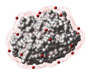
|
| Prev writevs_var | Home Up | Next icmmacros |